2.8 Mathematical Species

What species of mathematics is best suited for a task? Does it matter what species of mathematics we choose to build our models?

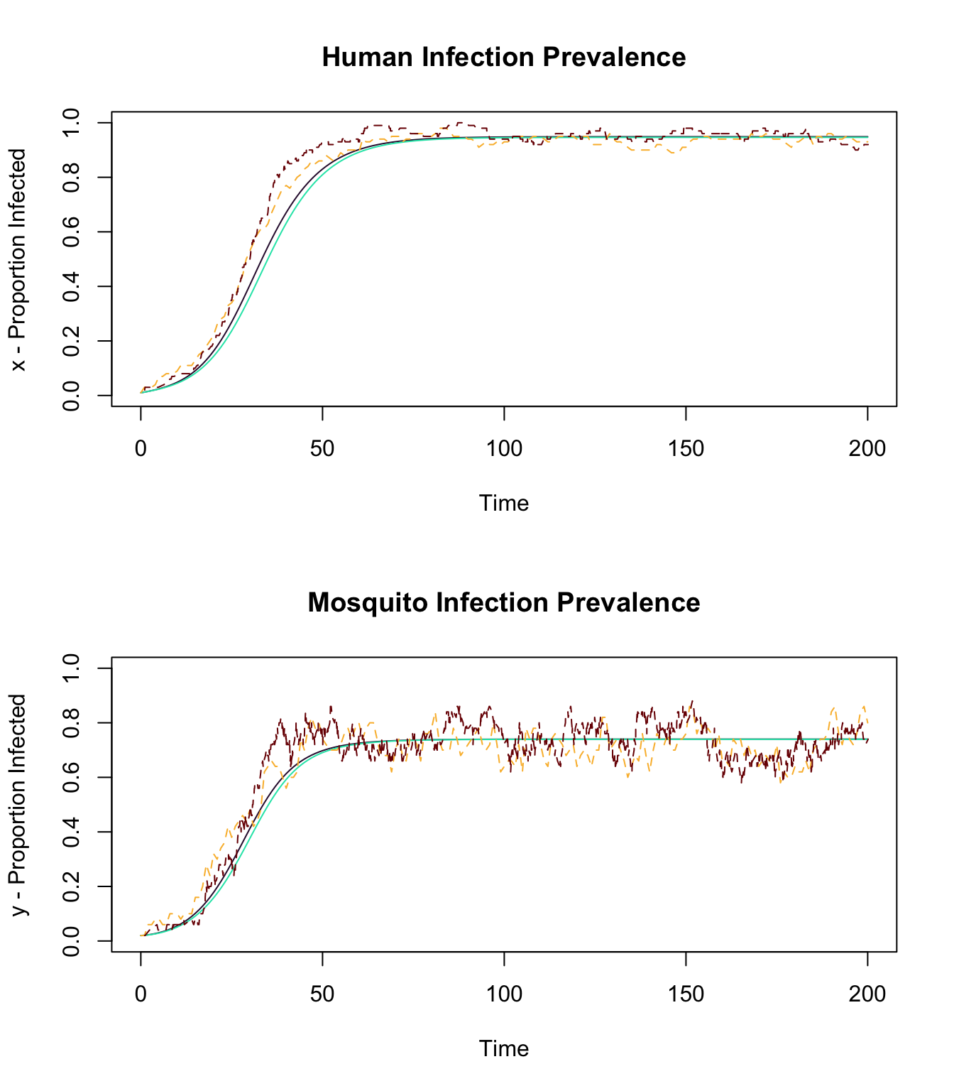
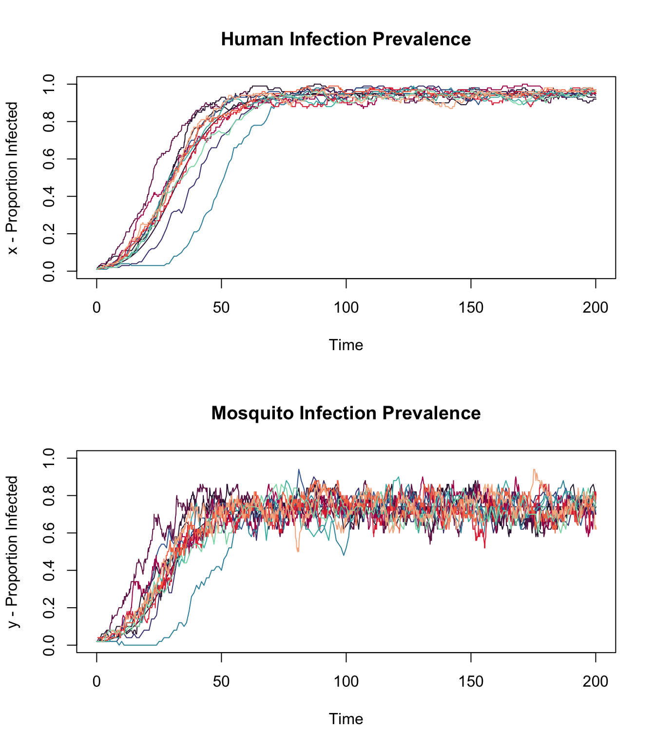
As we use models to help us understand malaria in some particular place, we are faced with some questions about to interpret the outputs of models. One of the reasons we presented deterministic and stochastic models in discrete-time and in continuous-time was to learn about about modeling by drawing attention to some of the differences – the models all represent the same process, but the outputs differ. Some of these differences are unsurprising and probably not important, but if we are to learn how to critically evaluate a model, we must pay attention to these differences. s

2.8.1 Deterministic Models

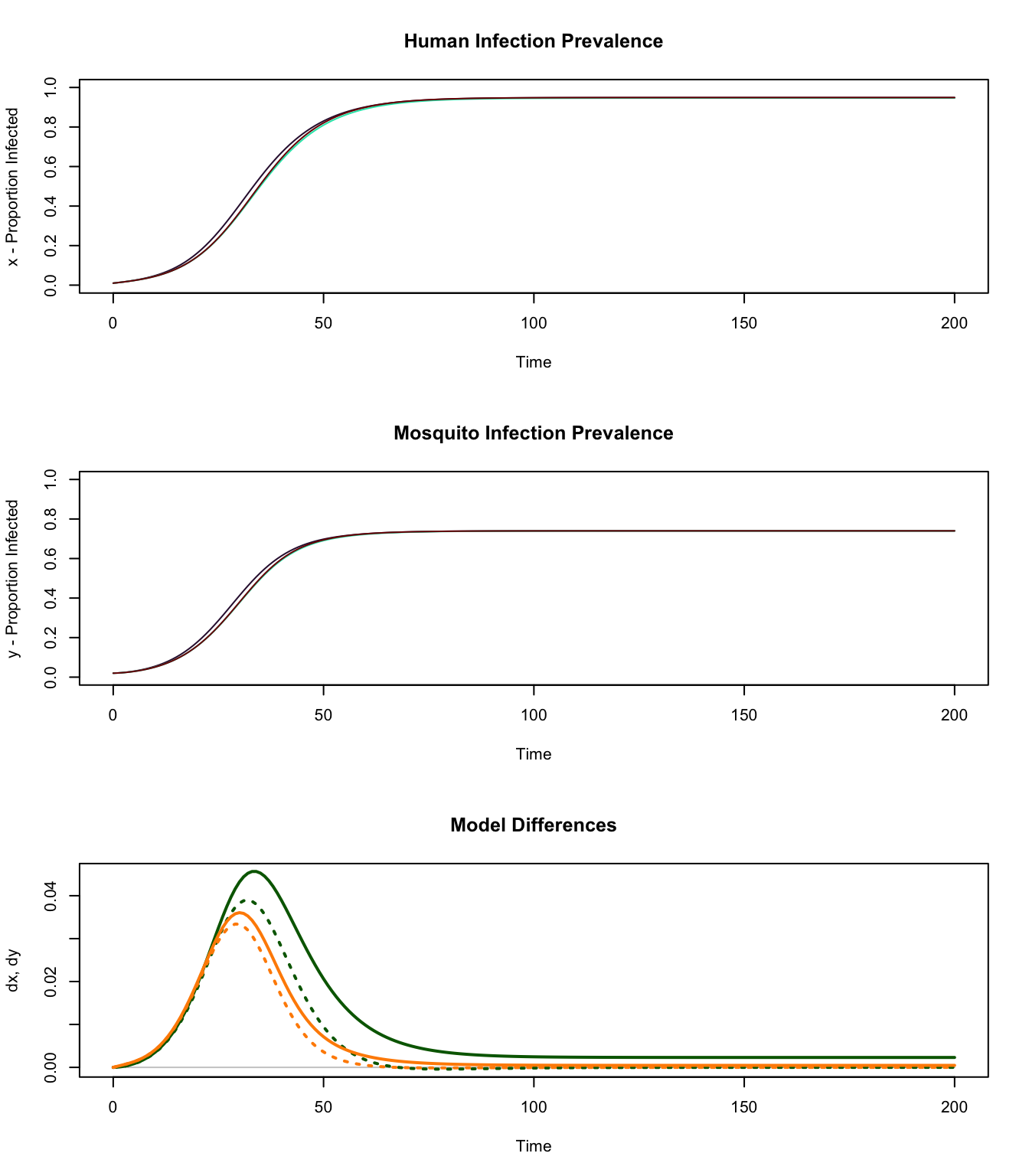
In the deterministic models, the variables over time are repeated in exactly the same way. If we changed a parameter or an initial condition, we would of course get different orbits. The discrete-time and continuous-time models differ slightly from each other. Some small differences will persist because we are dealing with non-linear processes.

In the following, we have plotted the outputs of all three deterministic models, and the differences between the continuous time and the two discrete-time models (bottom). The main difference between the two models is that malaria prevalence increases more slowly in the discrete-time models. The model ross_diffs_1 is slightly closer to the continuous time model.

How different are these two models? We could develop a formal distance metric to compare two models. First, since the variables in the continuous-time model is defined for every value of \(t\), but the discrete-time model is defined only for integer values of \(t\), we can only make comparisons for integer values of \(t.\) In the simulations above, we took care to output the values of both models at the same time points, so we can simply take the sum of squared differences:

ssd_2mods = function(m1, m2, norm=1){
  dx = sum((with(m1, x) - with(m2, x))^2) 
  dy = sum((with(m1, y) - with(m2, y))^2) 
  return((dx+dy)/norm) 
}

ssd_2mods(r_xde, r_dts, norm = length(r_xde$time))

## [1] 0.0003286306

Or the sub of their absolute values of the differences:

sabs_2mods = function(m1, m2, norm=1){
  dx = sum(abs(with(m1, x) - with(m2, x))) 
  dy = sum(abs(with(m1, y) - with(m2, y)))
  return((dx+dy)/norm) 
}

We can interpret this to mean that the average sum of differences is about 1.6%

sabs_2mods(r_xde, r1_dts, norm = length(r_xde$time))

## [1] 0.008878746

2.8.2 Stochastic Models

In stochastic models, the values of the variables differ each time we run the model.