2.6 Deterministic, Continuous Time

Differential equations.

In this section, we present a basic, deterministic, continuous-time model. After seeing the ross_dts models, this model will look and feel familiar. Instead of describing a difference over a fixed time step, we describe a derivative. The idea of derivative is usually introduced as the second new concept in any introduction to calculus. Instead of describing the fraction of a population that changes over any fixed time interval, the derivative describes change over an interval of time that is infinitesimally small.

To understand differential equations, you will need a background in calculus. If you’ve had a semester of calculus, you will have come across derivatives. Depending on how much calculus, you might not have solved differential equations. The point of this book is to introduce malaria analytics, so we will not be delving into mathematical theory or numerical methods very much.

In discrete-time, the equations could be written in this form:

\[ \begin{array}{rl} x_{t+1} - x_t &= F_x (x_t, y_t) \\ y_{t+1} - y_t &= F_y (x_t, y_t) \\ \end{array} \] The left hand side says “the difference in” \(x\) or \(y\) “over one time step is equal to” \(F_x\) or \(F_y,\) which are functions of the two variables. We can now ask what would happen if we sub-divided a day into \(n\) equal periods. In the limit as \(n\) goes to infinity, we replace the differences (terms on the left hand side) with derivatives. The differential equations are now written in this form:

\[ \begin{array}{rl} \frac{\textstyle{dx}}{\textstyle{dt}} &= F_x (x, y) \\ \frac{\textstyle{dy}}{\textstyle{dt}} &= F_y (x, y) \\ \end{array} \]

These differential equation models have the same components as the difference equations: variables, initial conditions, and parameters.

To compute anything, we will need to use numerical methods. Fortunately, R has a package to handle numerical methods for differential equations, called deSolve.

library(deSolve)

Here, we present and solve ross_xdea continuous time, deterministic model that is similar to Ross’s 2nd model [32].

2.6.1 `ross_xde`

Variables – In ross_xde, the dependent variables have the same meaning as in the ross_dts equations, but the independent variable. We now write an equation describing the fraction of humans and mosquitoes that are infected at each point in time.

Let \(x(t)\) be the fraction of people who are infected at time \(t,\) and \(0 \leq x(t) \leq 1.\)
Let \(y(t)\) be the fraction of mosquitoes who are infected at time \(t,\) \(0 \leq y(t) \leq 1.\)

Initial Conditions – As before, we will need to define initial conditions.

ross_xde_inits = c(x=0.01, y=0.01)

Parameters – In this model, the parameters describe rates of change.

Let \(r\) denote the fraction of people who clear infections after one day; \(0 < r < 1.\)
Let \(g\) denote the fraction of mosquitoes who die in one day; \(0 < g < 1.\)
Let \(a\) denote the fraction of mosquitoes who blood feed on a human in a day; \(0 < a < 1.\)
Let \(m\) denote the number of mosquitoes per human; \(m \geq 0.\)

# The parameters, as list 
ross_xde_par = list(
  r = 1/200, # The clearance rate for infections 
  g = 1/12,  # The mosquito daily death rate 
  a = 1/4,   # The mosquito human blood feeding rate 
  m = 0.5      # The number of mosquitoes per human
)

Equations – Finally, we put all this together into a mathematical statement that has translated the description of a process. There are four terms:

The fraction of humans who are infected is \(x\); infections clear at the rate \(r.\)
The fraction of mosquitoes who are infected is \(y\); mosquitoes die at the rate \(g.\)
The fraction of humans who are not infected is \(1-x\); infections occur at the rate \(m a y.\)
The fraction of mosquitoes who are not infected is \(1-y\); infections occur at the rate \(a x.\)

\[ \begin{array}{rl} dx/dt &= may(1-x) - r x\\ dy/dt &= ax(1-y) - g y \\ \end{array} \]

The form of the function that computes the derivatives in R is defined by deSolve

# INPUTS
# t - the current time 
# vars - the variables, as a named vector 
# pars - the parameters, as a list
# OUTPUTS
# the derivatives, as a list 
ross_xde = function(t, vars, pars){
  with(pars, 
    with(as.list(vars),{
    
      dxdt = m*a*y*(1-x) - r*x
      dydt = a*x*(1-y) - g*y
  
      return(list(c(dxdt, dydt)))
    })
  )
}

2.6.2 Rates vs. Proportions

The rates in differential equations can be compared to the proportions in discrete time systems. When the rates describe a change of state, a loss term for one of the variables, there are two easy interpretations. First, we consider the rate of loss of infected humans in a population, \(-rx.\) The core underlying process is exponential decay. If we followed a cohort, the waiting time for an individual to change states would follow an exponential distribution with rate \(1/r\). Second, after one day, the fraction that remains infected is \(e^{-r}\). If we set \(r=1/200,\) for example, the expected waiting time to clear an infection is 200 days. The rate of loss after one day is very close to, but slightly less than \(r\):

c(1/200, 1-exp(-1/200))

## [1] 0.005000000 0.004987521

2.6.3 Solutions

We now want to solve the initial value problem: given \(x(0)\) and \(y(0),\) can we find solutions \(x(t)\) and \(y(t)\)? To do so, we call deSolve::ode, which takes for arguments: the initial values, the points in time to ouput values of \(x(t)\) and \(y(t)\), a function that computes the derivatives, and the parameters:

deSolve::ode(ross_xde_inits, 0:5, ross_xde, ross_xde_par)

##   time          x          y
## 1    0 0.01000000 0.01000000
## 2    1 0.01128886 0.01172469
## 3    2 0.01279276 0.01363682
## 4    3 0.01453497 0.01577333
## 5    4 0.01654339 0.01817408
## 6    5 0.01884959 0.02088053

2.6.4 Computation & Visualization

For easy in working with these equations, we write a wrapper:

# INPUTS: 
# pars -- the parameter values, as a list
# x0   -- the initial value for x(t) 
# y0   -- the initial value for y(t) 
# tmax -- the largest value of t  
# dt   -- the interval for t 
# OUTPUT: 
# the output of ode as a data.frame 
ross_xde_solve = function(pars, x0=.01, y0=0.001, tmax=100, dt=1){
  tms = seq(0, tmax, by = dt)
  xy0 = c(x=x0, y=y0)
  data.frame(ode(xy0, tms, ross_xde, pars)) 
}

ode_out <- ross_xde_solve(ross_xde_par)

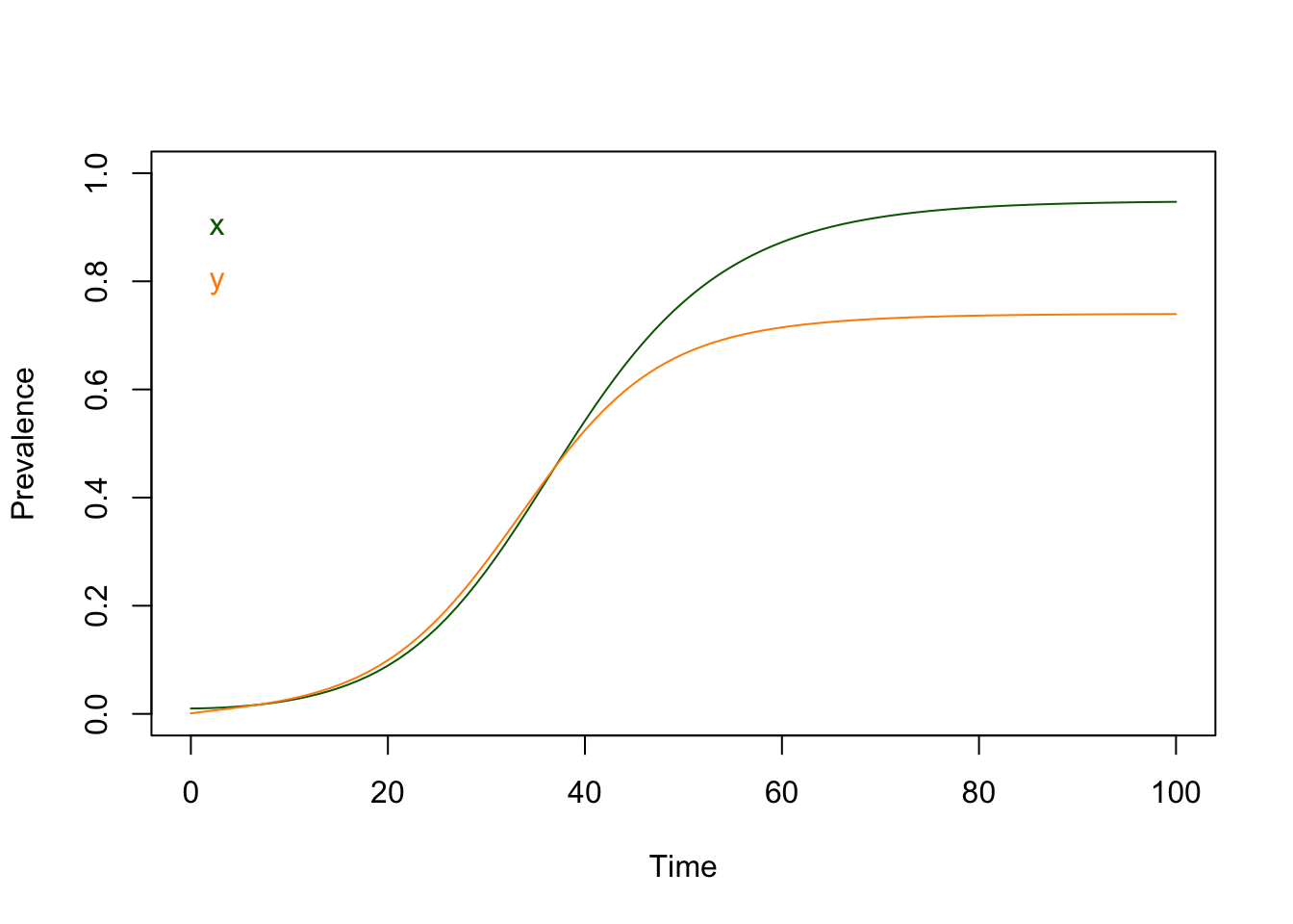
Because we have returned it as a data frame, the column names are time and x and y. We can plot the values using with().

plot_xy(ode_out)

These differential equations require

2.6.5 Steady States

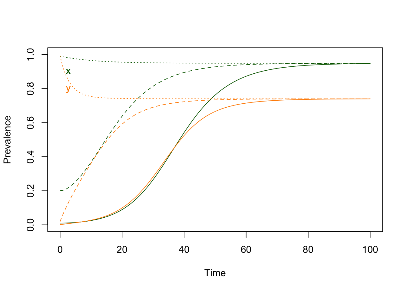
We can learn a bit more about how these equations behave by changing the initial values:

ode_out1 <- ross_xde_solve(ross_xde_par, x0=0.2, y0=0.02)
ode_out2 <- ross_xde_solve(ross_xde_par, x0=.99, y0=0.99)

plot_xy(ode_out)
plot_xy(ode_out1, lty=2, add=TRUE)
plot_xy(ode_out2, lty=3, add=TRUE)

We notice that the orbits all asymptotically approach the same values, regardless of where they started. Once there, they stay there.

2.6.6 Verification

We ought to be able to compute the value of these steady states: it is a value of \(x(t)\) and \(y(t)\) such that \(dx/dt=dy/dt=0.\) To find it, we set \(dx/dt=dy/dt=0\) and solve for \(x\) and \(y.\) One obvious value, once again, is \(x=y=0.\)

\[ \begin{array}{rl} 0 &= may(1-x) - r x\\ 0 &= ax(1-y) - g y \\ \end{array} \]

Solve the second equation for \(y\)

\[y = ax/(g+ax)\]

Substitute back into the first equation:

\[ma^2 (1-x) = r(g+ax)\] and solve.

\[x = \frac{\textstyle{m a^2 - rg}}{\textstyle{m a^2 + ra}}\]

Noting that \(m a^2 > rg\) must be a threshold condition, we write a function to compute the steady state using the formula we just derived:

ross_xde_steady_1(ross_xde_par)

##         x         y 
## 0.9487179 0.7400000

We check it against the other way, which involves running the system for a very long time.

de_eq <- ross_xde_solve(ross_xde_par, tmax=500, dt=5)
with(de_eq, c(x=tail(x,1), y=tail(y,1)))

##         x         y 
## 0.9487179 0.7400000

2.6.7 Thresholds

write me.

References

32.

Ross R. Some quantitative studies in epidemiology. Nature. 1911;87: 466–467.