2.3 Computation

A lot of analysis can be done with a pencil and paper, but this book is taking a computational approach. Here, we introduce some conventions that we will use to build software that can support robust analytics.

2.3.1 Functions

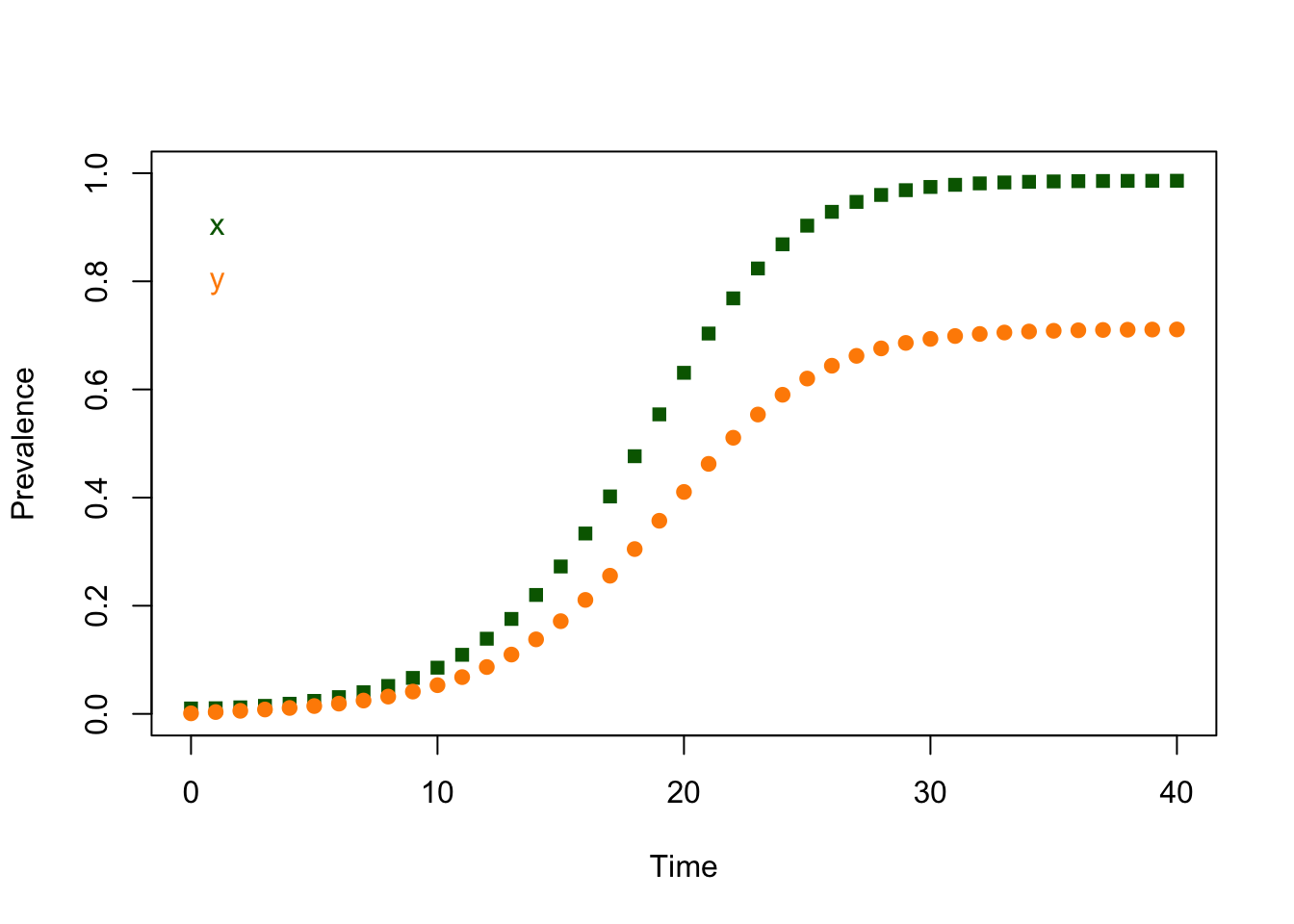
Computers are very good at repeating tasks, but if we want to get the computers to repeat tasks efficiently, we must write code that does it. One useful trick is to write functions that call other functions to expedite workflows. In this case, we want to write a function that solves the equations (i.e. that iteratively computes and stores the values) over some time interval:

# INPUTS
# pars - the parameters, as a list 
# x0   - the initial value of x
# y0   - the initial value of y
# t0   - the initial value of t
# tmax - the last value of t 
#
# OUTPUTS
# the values of the variables over time, as a list 
ross_dts_solve_1 = function(pars, x0=.01, y0 = 0.001, t0=0, tmax=100){
   xy = c(t=t0, x=x0, y=y0)
   xy_t = xy 
   for(t in (t0+1):tmax){
     xy = ross_diffs_1(xy, pars)
     xy_t = rbind(xy_t, xy)
   }
   return(list(time=xy_t[,1], x=xy_t[,2], y = xy_t[,3], last = xy)) 
}

We can write another function that plots the equations (i.e. that iteratively computes and stores the values) over some time interval:

# INPUTS
# xy_t - a list with elements named x, y, and time
# type - plot type:  "l" or "p" or "b"
# lty  - lty  
# add  - if TRUE, add to existing plot 
#
# OUTPUTS
# the values of the variables over time, as a list 
plot_xy = function(xy_t, type = "l", lty=1, add=FALSE){with(xy_t,{
  if(add == FALSE) 
  plot(time, x, "n", ylim = range(0, 1, y, x), ylab = "Prevalence", xlab = "Time")
  lines(time, x, type = type, lty=lty, col = "darkgreen", pch =15)
  lines(time, y, type = type, lty=lty, col = "darkorange", pch =19)
  text(0, 0.9, "x", col = "darkgreen", pos=4) 
  text(0, 0.8, "y", col = "darkorange", pos=4) 
})}

Now, we can define, solve and plot a model in a single line of code:

plot_xy(ross_dts_solve_1(ross_dts_makepars(), tmax=40), type="p") 

We’re not necessarily advocating that we write code this way. It’s not always easy to find and diagnose problems, or to repeat it. We shouldn’t do everything just because we can. This code does the same thing in a form that’s easier to follow:

params <- ross_dts_makepars()
output <- ross_dts_solve_1(params, tmax=40) 
plot_xy(output, type="p") 

2.3.2 Verification

If we’re going to take ourselves seriously, we want to get used to double checking everything to avoid making and propagating mistakes. One way to do this is to find two or more ways of computing the same thing, for verification.

If we’ve done everything right, we ought to get the same values for the steady states through our analysis and simulation.

The last values of \(x\) and \(y\) from the simulation are:

output$last[-1]

##         x         y 
## 0.9859663 0.7109837

The last values of \(x\) and \(y\) from evaluating ross_dts_steady_1() are:

ross_dts_steady_1(params) 

##         x         y 
## 0.9861386 0.7114286

It’s tempting to look at the printout and assume these two numbers are exactly equal, but when we deal with computers, everything gets computed and stored in some way. We can never be sure that a match will be be exact. We can simply sum up the absolute values of the differences:

sum(abs(output$last[-1] - ross_dts_steady_1(params)))

## [1] 0.0006171682

If we wanted to reduce this to a simple error check, we should pick a tolerance level – say \(10^{-9}\) – and then just ask if we are closer than that:

# INPUTS
# xy  - xy 
# par - a set of parameters for a ross_dts model 
# tol - a tolerance level 
#
# OUTPUTS
# boolean - 
ross_dts_checkit_1 = function(params, tmax=200, tol=1e-9){
  xy1 <- ross_dts_solve_1(params, tmax=tmax)$last[-1]
  xy2 <- ross_dts_steady_1(params)
  sum(abs(xy1 - xy2)) < tol
}

There are decisions to make. How long should we run the model? If we don’t run the simulation model for long enough, it will not have converged.

ross_dts_checkit_1(ross_dts_par, tmax=40)

## [1] FALSE

In this case, the model converges for the default value of tmax that we set:

ross_dts_checkit_1(ross_dts_par)

## [1] TRUE