2.4 Events and Counting

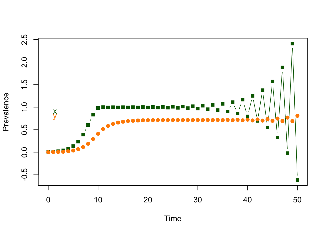
There is a problem with ross_diffs_1. If we set \(m\) too high, such that at some point \(m a y_t > 1,\) then the whole system eventually crashes:

ross_dts_par3 = ross_dts_makepars(m=12.4)
plot_xy(ross_dts_solve_1(ross_dts_par3, x0 = .01, y0=.001, tmax=50), "b") 

We need a good way of dealing with the problem that gave rise to this numerical instability. The question at hand is what fraction of people would become infected, on average, if the expected number of bites was \(may_t?\) Ideally, we want to return a proportion, even when \(may_t>1.\) We call this quantity – the fraction that gets infected in a day – the daily attack rate.

How should we compute the probability of infections if we expect to get exposed more than once?

2.4.1 On not not getting infected

In discrete time formulations, we must be very careful to ensure that we have formulated a proper model. How can we fix this problem? We have to go back and rethink the way we formulated our model. How does the probability of getting infected scale with the number of infective bites?

If we knew that there were exactly an integer number of bites, \(ma,\) then the proportion of people not getting infected would be those that didn’t get infected from any one of the bites, or \((1-y_t)^{ma}.\) There is, however, an even better way to think about this.

In a lot of cases like this, without any other information, we would assume that the number of bites, per person, would follow a Poisson distribution. It’s actually easier to say who doesn’t get infected, and that’s the zero term of a Poisson, \(e^{-may_t}.\) The probability of getting infected is the complement of the probability of getting at least one bite, or

\[1 - e^{-m a y_t}\]

2.4.2 ross_dts_2

Equations

Our variables, initial conditions, and parameters are all defined in the same way as ross_diffs_1, but now our equations have changed:

\[\begin{equation} \begin{array}{rl} x_{t+1} &= x_t - s x_t + (1-e^{-m a y_t}) (1-x_t) \\ y_{t+1} &= y_t - u y_t + a x_t (1 - y_t) \\ \end{array} \tag{2.6} \end{equation}\]

As before, we write a function to numerically solve the discrete time system:

# INPUTS
# xy      - current variables, as a named vector
# params  - the parameters, as a list
#
# OUTPUTS
# the updated values of the variables, as a named vector
ross_dts_2 = function(xy, params){with(as.list(xy), with(params,{
  xn = x - s*x + (1-exp(-m*a*y))*(1-x) 
  yn = y - u*y + a*x*(1-y) 
  t=t+1
  return(c(t=t, x=xn, y=yn))
}))}

Once again, we can wrap a function around the solver so that it’s easier to use the code:

# INPUTS
# pars - the parameters, as a list 
# x0   - the initial value of x
# y0   - the initial value of y
# t0   - the initial value of t
# tmax - the last value of t 
#
# OUTPUTS
# the values of the variables over time, as a list 
ross_dts_solve_2 = function(pars, x0=.01, y0 = 0.001, t0=0, tmax=100){
   xy = c(t=t0, x=x0, y=y0) 
   xy = c(t=0, x=x0, y=y0) 
   xy_t = xy 
   for(t in (t0+1):tmax){
     xy = ross_dts_2(xy, pars)
     xy_t = rbind(xy_t, xy)
   }
   return(list(time=xy_t[,1], x=xy_t[,2], y = xy_t[,3], last = xy)) 
}

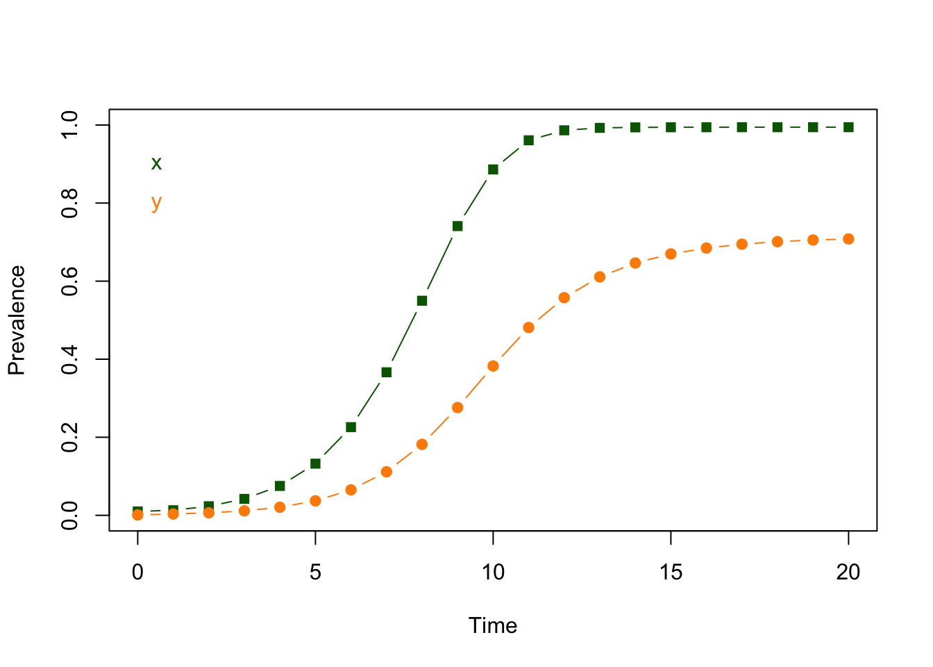
Now, we can visualize the output using code we’ve already written, and can see that we have fixed our stability problem.

plot_xy(ross_dts_solve_2(ross_dts_par3, x0 = .01, y0=.001, tmax=20), "b") 

Verification

For verification, we want a method to solve things two different ways. If we want to compute the steady state, we’re stuck with the problem of solving this equation:

\[(1-e^{-m a^2 x/(u + a x)}) (1-x) = sx\]

It’s surprisingly easy to write down equations, like this one, that we can’t solve with pencil and paper. We can still find a way of computing the steady state, but we have to write R code that solves for \(x\) numerically.

# INPUTS
# par - the model parameters, as a list 
#
# OUTPUTS
# the steady state values of x and y 
ross_dts_steady_2 = function(pars, tol=1e-10){with(pars,{
   f_xx = function(x, pp){with(pp,{
     xx = (1 - exp(-m*a^2*x/(u+a*x)))*(1-x) - s*x
     y = a*xx/(u+a*xx)
     yy = u*y + a*xx*(1-y) 
     return(xx^2 + yy^2)
   })}
   xx = optimize(f_xx, c(0,1), pp=pars, tol = tol)$min
   yy = a*xx/(u+a*xx) 
   c(xx, yy)
})}

Finding the equilibrium this way, we get:

ross_dts_steady_2(ross_dts_par3)

## [1] 0.9944158 0.7131415

Second, by getting the solution after many iterations.

ross_dts_solve_2(ross_dts_par3, x0=.1, y0=.05, tmax=300)$last[-1]

##         x         y 
## 0.9944158 0.7131415

By inspection, these two numbers are very close, but not exactly matching. Once again, we want to ensure that our code does not have any mistakes, so we write a function to verify our results. We set a term that describes an acceptable tolerance for computational errors, and ask if we’re at least that close.

# INPUTS
# xy     - xy 
# par    - a set of parameters for a ross_dts model 
# tmax   - maximum runtime for ross_dts_solve_2 
# st_tol - tolerance for ross_dts_steady_2
# tol    - desired tolerance for verification
#
# OUTPUTS
# boolean - 
ross_dts_checkit_2 = function(params, tmax=300, st_tol=1e-10, tol=1e-7){
  xy1 <- ross_dts_solve_2(params, tmax=tmax)$last[-1]
  xy2 <- ross_dts_steady_2(params, tol=st_tol)
  sum(abs(xy1 - xy2)) < tol
}

Do the two answers differ by less than \(10^{-7}\)?

ross_dts_checkit_2(ross_dts_par3)

## [1] TRUE

It’s a little unsatisfying to get numerical errors, but machines don’t do exact computation easily. We’re interested in getting as close as we need to get without doing a lot of work that would, in the end, never make a difference. The operating principle here is that we need to be sure that our code is doing what we think it should, and that it is giving answers that are close enough.

Also of interest, discrete time model ross_diffs_2 was implemented in a Google Sheet.