library(ramp.xds)
library(ramp.library)SimBA: A Demo
SimBA was designed to support malaria analytics by facilitating human interactions about malaria that rely on dynamical systems describing malaria. To accomplish this, SimBA has developed functions and algorithms that make it easy to setup, solve, visualize, analyze, fit, and use the models. SimBA lowers the human and computing costs of model building, computation, and analysis.
To illustrate the capabilities of SimBA, we do the following:
Build a dynamical system to describe malaria
Solve it
Visualize the outputs
Fit the model to data
Compute the burden of malaria and the avertible burden
Compute thresholds
Analyze scaling relationships
Add a forecast to the fitted model
Predict malaria prevalence by diagnostic, age, and time of year
Make a plan by evaluating and comparing the likely outcome of interventions
Adapt
A feature of SimBA is its capacity to scale complexity. The software is modular, flexible, and extensible making it possible to build models that are more complex and replicate some of these processes. The exception to this rule is model fitting, which has its own set of perils and pitfalls.
Build
We assume our audience knows something about mathematical models for malaria. SimBA handles models for malaria epidemiology, transmission dynamics, and control that were formulated as dynamical systems. The software is capable of supporting systems of differential equations or discrete time systems. To build models, we need two packages:
These two software packages have several published models for malaria and mosquito ecology. For the purposes of this demonstration, we will start with a compartmental model for malaria called the SIP model. For mosquitoes, we use the SI model. Setting up a model is as easy as calling xds_setup and passing the names of the modules:
model <- xds_setup(Xname = "SIP", MYname = "SI")The object that was returned, model, is called a ramp.xds model object. The object has been set up to handle a lot of complexity that we may not need.
names(model) [1] "model_name" "xde" "xds"
[4] "frame" "forced_by" "nVectorSpecies"
[7] "nHostSpecies" "nPatches" "nHabitats"
[10] "nStrata" "nOtherVariables" "terms"
[13] "ML_interface" "XY_interface" "variables"
[16] "Xname" "XH_obj" "MYname"
[19] "MY_obj" "Lname" "L_obj"
[22] "V_obj" "resources_obj" "forcing_obj"
[25] "health_obj" "vector_control_obj" "outputs"
[28] "max_ix" If we type the name, it will tell us the basic features of the model:
model[1] HUMAN / HOST
[1] # Species: 1
[1]
[1] X Module: SIP
[1] # Strata: 1
[1]
[1] VECTORS
[1] # Species: 1
[1]
[1] MY Module: SI
[1] # Patches: 1
[1]
[1] L Module: trivial
[1] # Habitats: 1 Solve
model <- xds_solve(model, Tmax=180) Visualize
par(mfrow = c(2,1))
xds_plot_EIR(model)
xds_plot_PR(model)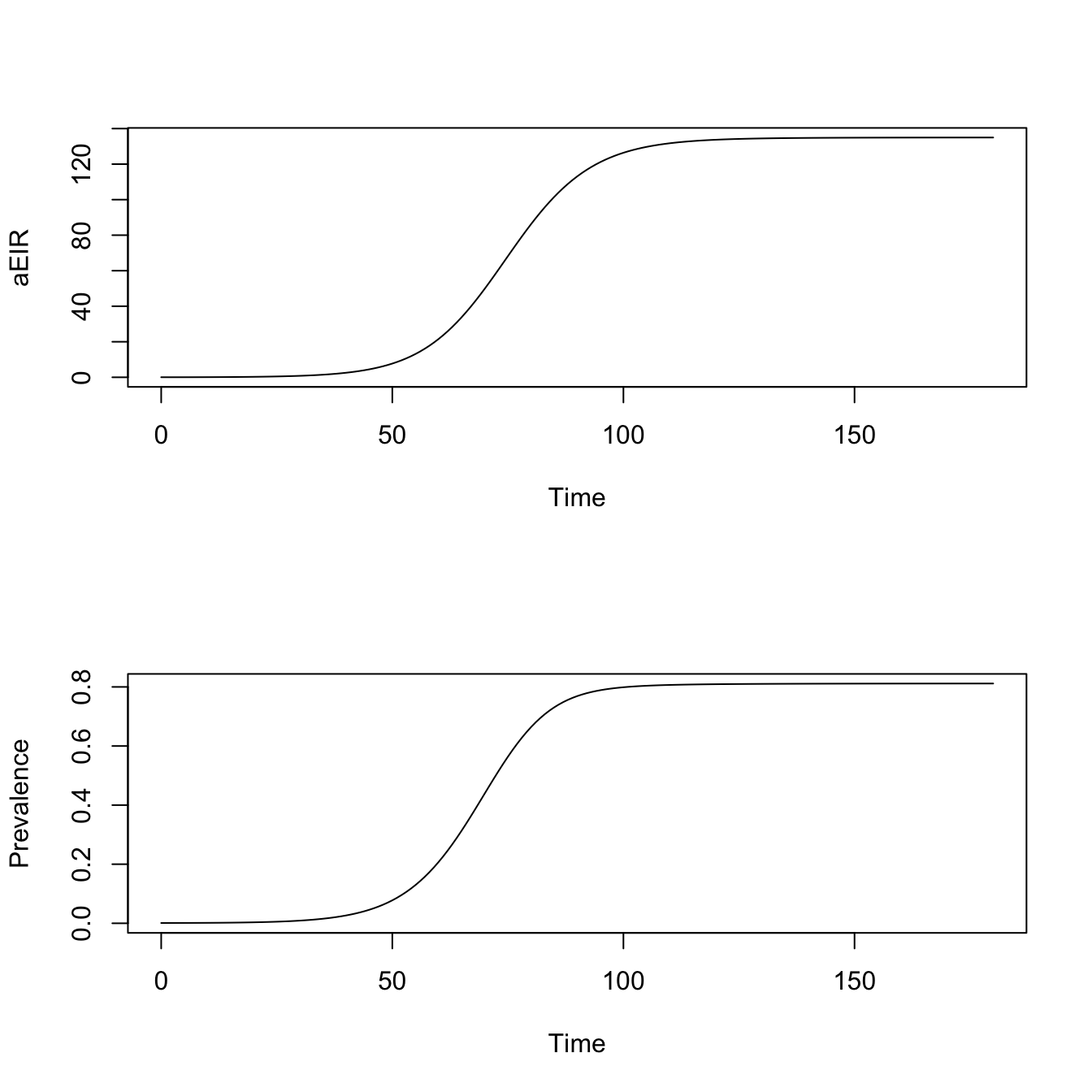
Fit
Forcing and functions in SimBA
Time series
Set up Forcing
model <- xds_fit_model(model) Burden
Scaling
library(ramp.work)Loading required package: ramp.controlLoading required package: MASSmodel <- xds_scaling(model) Thresholds
model <- xds_thresholds(model) Forecast
model <- xds_forecast(model)