Time Spent

Author

Affiliation

University of Washington

For basic malaria analytics, SimBA relies on the concepts of time spent and time at risk [1]. Here, we look at options for setting up a time spent matrix.

Also see: Time at Risk and Malaria Theory: Time Spent at Risk

Time Spent Matrix

Let \(\Theta\) denote the time spent matrix. A time spent matrix is constructed by considering the travel patterns of each population stratum. Each column in \(\Theta\) represents the first \(p\) elements of a time spent vector, \(\theta_j\) where \(j\in 1,2,\ldots, p\). By design, the time spent matrix does not include time spent during travel or not at risk:

\[\begin{equation} {\Theta} = \left[ \begin{array}{ccccc} i=1&i=2&i=3&\cdots&i=n \\ \boxed{ \begin{array}{c} {\Theta}_{1,1} \\ {\Theta}_{2,1} \\ {\Theta}_{3,1} \\ \vdots \\ {\Theta}_{p,1} \\ \end{array}} & \boxed{ \begin{array}{c} {\Theta}_{1,2} \\ {\Theta}_{2,2} \\ {\Theta}_{3,2} \\ \vdots \\ {\Theta}_{p,2} \\ \end{array}} & \boxed{ \begin{array}{c} {\Theta}_{1,3} \\ {\Theta}_{2,3} \\ {\Theta}_{3,3} \\ \vdots \\ {\Theta}_{p,3} \\ \end{array}} & \boxed{ \begin{array}{c} \cdots \\ \cdots \\ \cdots \\ \ddots \\ \cdots \end{array}} & \boxed{ \begin{array}{c} {\Theta}_{1,n} \\ {\Theta}_{2,n} \\ {\Theta}_{3,n} \\ \vdots \\ {\Theta}_{p,n} \\ \end{array}} \end{array} \right] \end{equation}\]

The columns should sum up to less than one. By convention, the implementation in ramp.xds handles travel (time outside of any patch) separately. If the columns sum to a number less than one, it should reflect time spent in places where they are not at risk, such as automobiles, or office buildings.

The time spent matrices are designed for short-term projections, so population changes due to human births, deaths, and migration are either assumed to be small, or they are dealt with through stratification.

Basic Setup

The time spent matrix can be configured in basic setup.

library(ramp.xds)
library(ramp.func)
library(ramp.qa)

Default Options

The default setting for xds_setup is that all time is spent in the patch where a person resides. If \(N_p=1\) then the time spent matrix for one stratum is:

model <- xds_setup()
get_timespent_matrix(model)

     [,1]
[1,]    1

For multiple strata:

model <- xds_setup(residence = c(1,1,1), HPop = c(100, 900, 200))
get_timespent_matrix(model)

     [,1] [,2] [,3]
[1,]    1    1    1

Residence Vector

If the user sets nPatches and passes a residence vector, the time spent matrix is identical to the residence matrix:

model <- xds_setup(nPatches =3, residence = c(1,1,2,2), 
                   HPop = c(20, 80, 100, 900))
get_timespent_matrix(model)

     [,1] [,2] [,3] [,4]
[1,]    1    1    0    0
[2,]    0    0    1    1
[3,]    0    0    0    0

Matrix

M = matrix(c(.9, .07, .03, .95, .02, .03, 0.01, .98, 0.01, 0.1, .8, .1), 3, 4)
M

     [,1] [,2] [,3] [,4]
[1,] 0.90 0.95 0.01  0.1
[2,] 0.07 0.02 0.98  0.8
[3,] 0.03 0.03 0.01  0.1

If the matrix is passed to setup_timespent then (after passing checks) it becomes the time spent matrix.

model <- setup_timespent(M, model)
get_timespent_matrix(model)

     [,1] [,2] [,3] [,4]
[1,] 0.90 0.95 0.01  0.1
[2,] 0.07 0.02 0.98  0.8
[3,] 0.03 0.03 0.01  0.1

model <- xds_setup(nPatches = 3, residence = c(1,1,2,2), 
                   HPop = c(20, 80, 100, 900), TSoptions = M)
get_timespent_matrix(model)

     [,1] [,2] [,3] [,4]
[1,] 0.90 0.95 0.01  0.1
[2,] 0.07 0.02 0.98  0.8
[3,] 0.03 0.03 0.01  0.1

At Home

The at_home option calls make_timespent_at_home has two optional arguments:

at_home is the fraction of time spent at home
not_at_risk — the columns sum to 1-not_at_risk
time away from home is evenly divided among the non-resident patches

Note that the following is modifying the time at risk matrix. It leaves the residence unchanged:

options = list(name = "at_home", at_home = .95, not_at_risk =0.01)
model <- setup_timespent("at_home", model, options)
get_timespent_matrix(model)

     [,1] [,2] [,3] [,4]
[1,] 0.95 0.95 0.02 0.02
[2,] 0.02 0.02 0.95 0.95
[3,] 0.02 0.02 0.02 0.02

To get the same thing during basic setup:

model <- xds_setup(nPatches = 3, 
                   residence = c(1,1,2,2), 
                   HPop = c(20, 80, 100, 900), 
                   TSoptions = options)
get_timespent_matrix(model)

     [,1] [,2] [,3] [,4]
[1,] 0.95 0.95 0.02 0.02
[2,] 0.02 0.02 0.95 0.95
[3,] 0.02 0.02 0.02 0.02

`xy`

The setup_timspent.xy option grabs the residence vector and then calls make_timespent_xy with options:

xy — the \(x\) and \(y\) coordinates of each patch
residence — use get_residence
stay — the fraction of time spent at home
kern — a function to weight patches by distance, any information on the xds model object (e.g. human population density), or any options passed to the function. The form of the function is: \[F_k(d, M, O)\] where M is the model object and O is options is a named list.
k_opts — options, passed as a named list (to setup_timepent(name = "xy", ...)).

In the following example, we generate 10 random patch locations, as \(x,y\) coordinates, in a \(10 \times 10\) box centered at 0. The human population has 10 strata: one for each patch. Individuals spend, on average, around 80% of their time at home (drawn from a beta distribution). The remaining time is allocated to points by a distance function: \[F_K(d) = e^{-(d-3)^2}.\] The example is meant to be illustrative, not realistic.

x = runif(10, -5, 5)
y = runif(10, -5, 5)
xy = data.frame(x=x, y=y)
stay=rbeta(10, 8, 2)
HPop = rnbinom(10, mu=1000, size=.5)
kern = function(d, model, options){exp(-(d-3)^2)}
options = list(name="xy", xy=xy, kern=kern, stay=stay) 
model <- xds_setup(nPatches = 10, 
                   residence = 1:10, 
                   HPop = HPop, 
                   TSoptions = options)
get_timespent_matrix(model)->M
plot_connectivity_graph(M, xy, mn=0.01, 
                        labels = signif(rowSums(M), 3),
                        arr.pos=0.8, scl=5)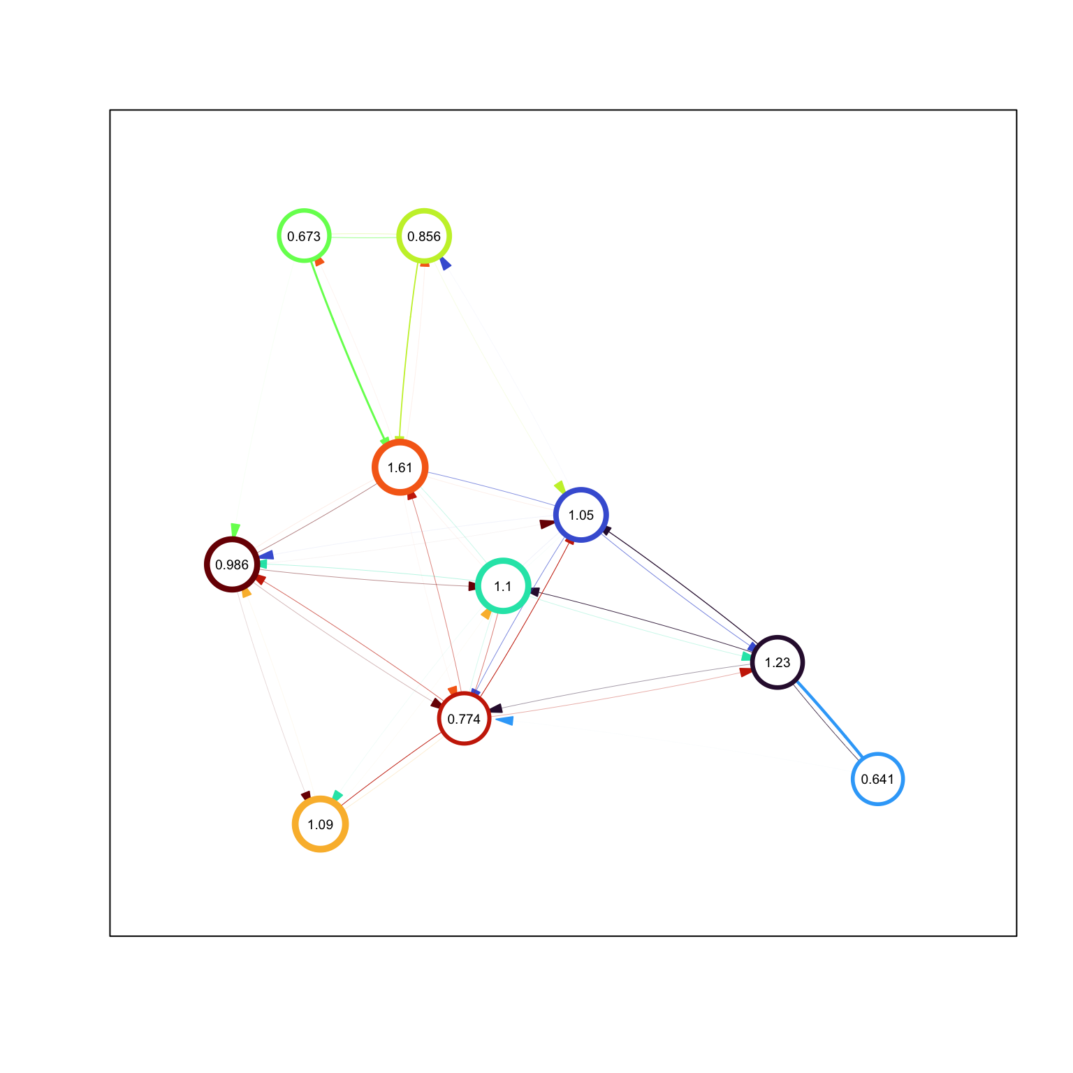

In developing models of real systems, we assume that time spent around home, the non-resident elements of a time spent matrix, are related to work, school, health, religion, food, recreation, and houshehold or administrative tasks [2]. To handle these, the definition of kern passes both the model object and the setup options list, so any information available from one of these sources can be used to compute time spent around home.

Ambient Population Density

A good way to check models for time spent away from home is to compute ambient population density:

\[A = \Theta \cdot H\] Note that the resident population density is:

\[H_p = J \cdot H\]

The tourist index is a measure of the ratio of ambient to resident density:

\[A/H_p\]

References

Wu SL, Henry JM, Citron DT, Ssebuliba DM, Nsumba JN, C HMS, et al. Spatial dynamics of malaria transmission. PLoS Computational Biology. 2023;19: e1010684. doi:10.1371/journal.pcbi.1010684

Perkins TA, Garcia AJ, Paz-Soldán VA, Stoddard ST, Reiner RC, Vazquez-Prokopec G, et al. Theory and data for simulating fine-scale human movement in an urban environment. J R Soc Interface. 2014;11. doi:10.1098/rsif.2014.0642