library(ramp.xds)
library(ramp.control)Mass Treatment
Malaria models in SimBA are set up to handle mass treatment. Unlike many other interventions, treating malaria modifies the state space describing infection, so the effects of mass treatement are implemented in the XH component.
Each X module handles treatment differently, but many of them have a port to handle mass treatment. By convention, the ports are called
mdafor mass drug administration (MDA). The population is treated without testing.msatfor mass screen and treat (MSAT), which involves testing (usually with an RDT) and treating those who test positive.
If the port exists, then it is in the skill set. For example, we can check and see if mda is in the skill set of the SIS model:
skill_set_XH("SIS")$mda[1] TRUESimilarly for MSAT:
skill_set_XH("SIS")$msat[1] TRUETo understand how the mda ports works, we can take a look at the SIS model. The relevant lines in dXHdt.SIS are these:
r_t <- r + mda(t) + msat(t)
dI <- foi*(H-I) - r_t*I + D_matrix %*% I
During set up, the functions mda and msat are assigned the same values.
In the SIS X module, mass treatment clears infections, but since there is no chemo-protected class, treated people become susceptible. The SIS implementation, in math notation, looks like this:
\[ \begin{array}{rl} \frac{\textstyle{dH}}{\textstyle{dt}} &= B(t) - {\cal H} \cdot H \\ \frac{\textstyle{dI}}{\textstyle{dt}} &= h S - (r + \xi(t)) I - {\cal H} \cdot I \end{array} \]
The function call to \(\xi(t)\) is called mda. To see the actual function call, look at dXdt.SIS in human-SIS.R in ramp.xds.
Basic Setup
In the SIS model, implemented in a generalized form with demographic change, setup creates a function \(\xi(t)\) to simulate mass treatment, but then sets it equal to zero (i.e. the function F_zero).
model <- xds_setup_eir(Xname = "SIS", eir=1/365,
                          season_par = makepar_F_sin())
model <- xds_solve(model, times = c(3650, 3650))
model <- last_to_inits(model)
model <- xds_solve(model,Tmax=730)
xds_plot_PR(model)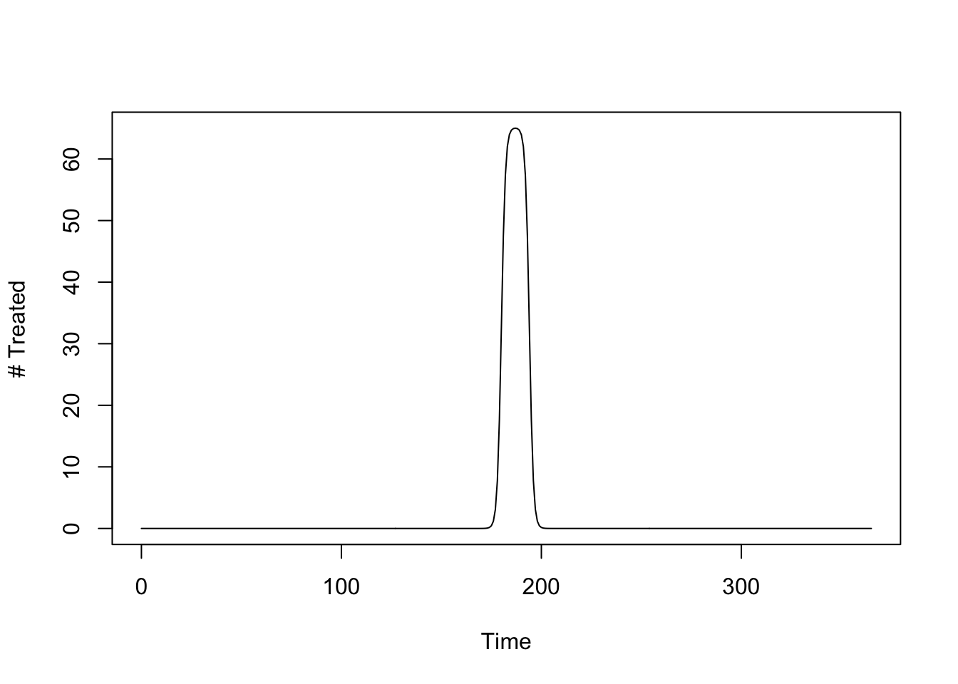
Advanced Setup
There is no basic setup option that would allow a user to configure mass treatment at setup: it must be done through advanced setup. In a nutshell, a model gets modified after basic setup.
We do this by calling setup_mass_treat_events and passing the start time (start - a Julian date), the number of days it will take to treat (span), the fraction treated (frac_treated) and whether screening is required before testing (test).
start = 180
span = 10
frac_treated = 0.9
test = FALSE
model <- setup_mass_treat_events(model, start, span, frac_treated, test)
The function F_treat(t) should return a function that describes the number of people treated each day over a simulation. This enforces a kind of discipline for malaria analysts for whom mass treatment must be costed. The question it begs is how much does it cost to send out a team for some number of days with the capacity to treat some number of people each day, and how many people they actually treat.
The following function sets up mass drug administration to treat 65 people, per day, for 14 days. The model says we are sending out a team that has the capacity to treat around 910 people (actually, \(\approx 911.7\)).
mda_par <- makepar_F_sharkfin(D = 180, L = 14, uk = 1, dk=1, mx = 1/14)
mda <- make_function(mda_par)
integrate(mda, 0, 365)$value -> capacity
capacity
[1] 1.001825The number treated over time looks like this:
tt <- seq(0, 730, by = 1)
plot(tt, mda(tt), type = "l", xlab = "Time", ylab = "# Treated")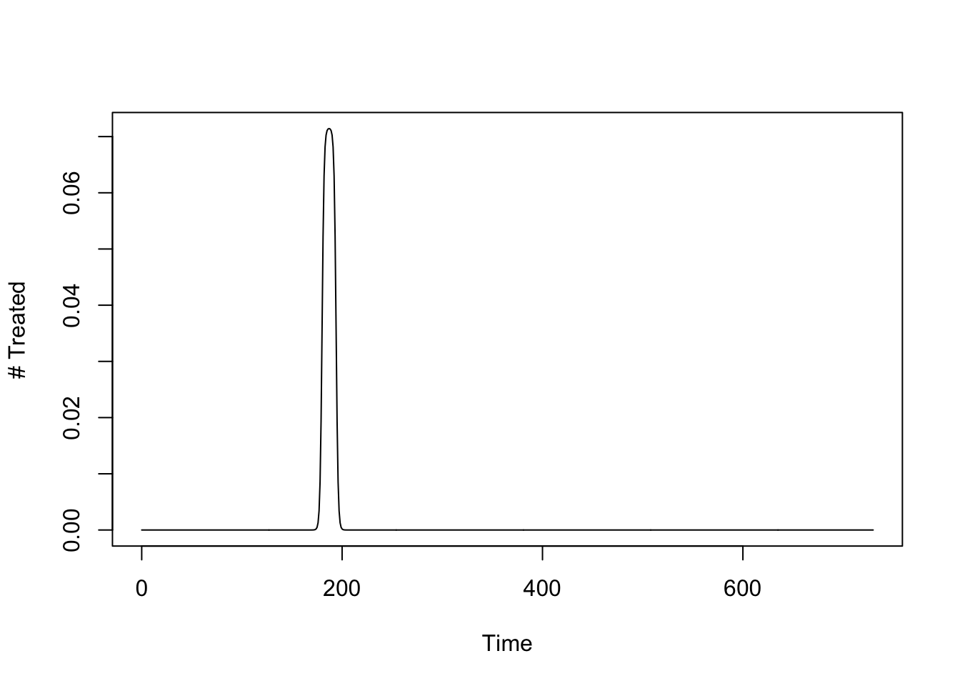
In this case advanced setup just means modifying the function F_treat. A function call to setup_mda would make it easier, but this is what that setup call would do:
We want to compare our model with mda to the model without, so we clone the base model and modify the clone, then solve it:
mda_model <- model
mda_model$XH_obj[[1]]$mda = mda
mda_model$XH_obj[[1]]$mda(100)
[1] 0mda_model <- xds_solve(mda_model, Tmax=730)Now, we can compare the two models. The orbit for MDA is in darkred:
xds_plot_PR(model)
xds_plot_PR(mda_model, clrs = "darkred", add=TRUE)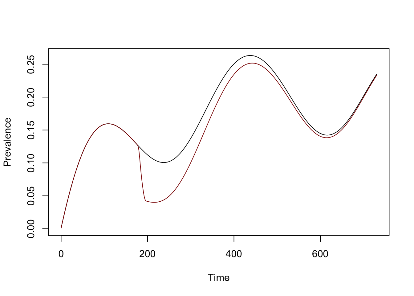
Capacity vs. Outcome
The fraction of people is lower than 91%. In the default setup, \(H\) is set to 1,000 people. The term in the model describes treatment of infected individuals at a per-capita rate of \(65/H,\) and with \(H=1000\), in the end about 59.8%, or \(1-e^{-900/h}\), or \(598\) unique individuals get treated. The functional forms could be interpreted to reflect a reality that a team will find it increasingly difficult to find individuals who have not been treated.
frac = 1-exp(-capacity)
frac
[1] 0.6327915Calibration
If a team is more technically efficient, an analyst can set up the analysis differently, understanding how the math works, how the costs work. Suppose we want to send out a team to treat 90% of the population, and the malaria program knows how much it costs. Now, the analyst must configure a model to treat 90%.
This configures a model to start mda on day \(90\) and 200 people a day (\(mx=200\)), for a week \((L=7),\) or about \(1,400\) people. The function shape is tapered at both ends, so the area under the curve is not exact.
mda_par <- makepar_F_sharkfin(D = 90, L = 7, uk=2, dk=2, mx = 1/5)
mda <- make_function(mda_par)
integrate(mda, 0, 365)$value -> capacity
capacity
[1] 1.403942In a population of \(1,000\), only about \(776\) people get treated.
frac = 1-exp(-capacity)
frac
[1] 0.7543733We can develop a function that makes all this easier:
cap2frac = function(capacity, duration=7, H=1000){
   mda_par <- makepar_F_sharkfin(D = 90, L = duration, uk = 1, dk=1, mx = capacity)
   mda <- make_function(mda_par)
  integrate(mda, 0, 365)$value -> capacity
  c(capacity = capacity, frac = 1 - exp(-capacity/H))
}
The function does the math:
cap2frac(200, 7, 1000) capacity frac
1497.9864119 0.7764201 Now suppose I want to treat 90% of the population. I can simply adjust the number treated, per day, until I get 90% treated in a week:
cap2frac(306, 7, 1000) capacity frac
2291.9192103 0.8989277 Now we can set up a new model:
alpha = 0.95
L = 7
mda_par <- makepar_F_sharkfin(D = 90, L = L, uk = 1, dk=1, mx = -log(1-alpha)/L)
mda <- make_function(mda_par)
mda_model1 <- model
mda_model1$XH_obj[[1]]$mda = mda
mda_model1 <- xds_solve(mda_model1, Tmax=730)
…and we can visualize all three models:
xds_plot_PR(model)
xds_plot_PR(mda_model, clrs = "darkred", add=TRUE)
xds_plot_PR(mda_model1, clrs = "purple", add=TRUE)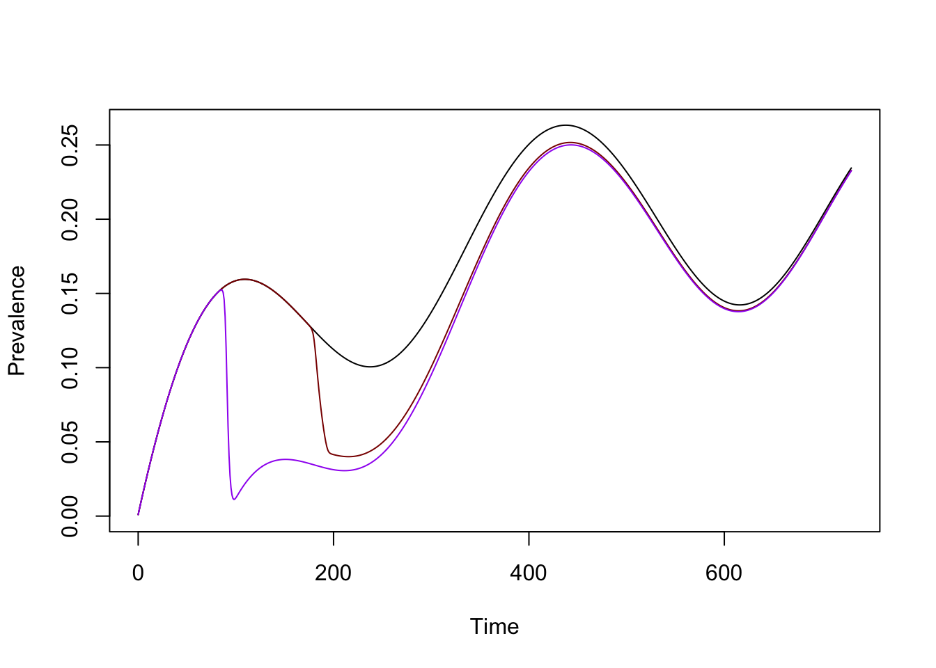
SIP
In the SIP model,…