Scenario Planning

In the following vignette, we use a model for scenario planning, which involves several steps:

Set up a model
Fit it to data –
Knowing the timing of vector control, we want to evaluate its impact:
- What was the effect of ITNs?
- What was the effect of IRS?
To evaluate plans for the future, we need a business-as-usual forecast
Against that BaU scenario, we can now evaluate:
- What should we expect from ITNs?
- What should we expect from IRS?
- What should we expect from mass drug administration?

Set up a model

The first step is to set up a model.

Here, we are starting with the simple SIS compartment model. This is one of the base models in ramp.xds:

library(ramp.xds)

model <- xds_setup_cohort(Xname = "SIS", 
                          eir = 2/365, 
                          season_par = makepar_F_sin(), 
                          trend_par = makepar_F_spline(c(0:9)*365, rep(1,10)))

model <- xds_solve_cohort(model, 3650, 3650)
model <- last_to_inits(model)
saveRDS(model, "model.rds")

At this point, some of the parameter values have been chosen arbitrarily, just to set up the structures we want to fit. Even so, we can visualize the outputs:

model <- xds_solve_cohort(model, A=2, da=10)
xds_plot_PR(model)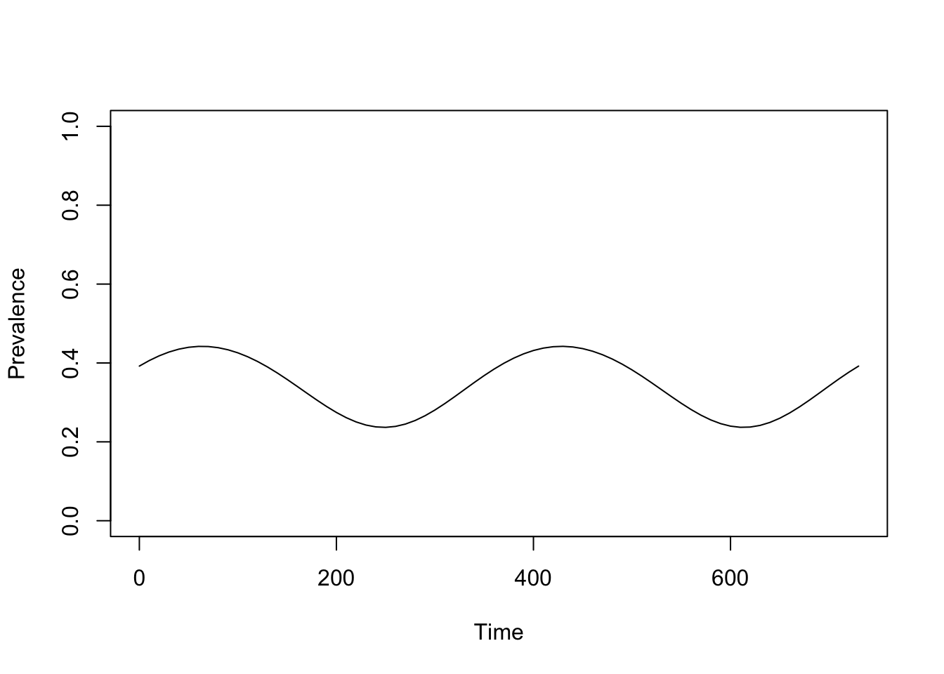

Fit it to data

Background – Our goal is to develop reliable malaria intelligence – estimates of malaria transmission that are ready for simulation-based analytics. In malaria analytics, we use PfPR as the pivotal metric, but most of the data we have is from clinical surveillance [1–3]. A concern with the clinical surveillance data is that it is collected passively, so it is impossible to design a study to validate clinical data. If we want to trust it, we need to develop algorithms that use the surveillance metrics to make testable predictions about the value of research metrics. The research metric of choice is the PfPR [1–3].

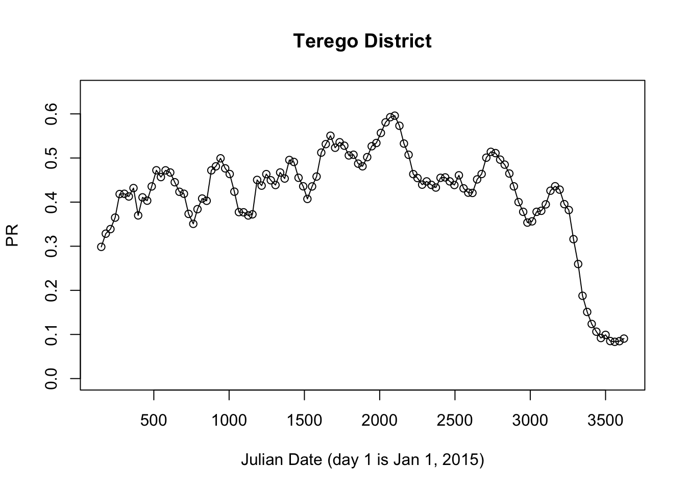
We have done this in Uganda. Here, we do some analysis using a time series of imputed PfPR data for Terego District, West Nile, Uganda.

library(ramp.uganda)
prts <- get_district_pfpr("Terego District")
with(prts, {
  plot(jdate, pfpr, ylim = c(0,0.65), main = "Terego District", xlab = "Julian Date (day 1 is Jan 1, 2015)", ylab = "PR") 
  lines(jdate, pfpr)
})

The next step we do is to develop a basic understanding of malaria prevalence over time by fitting a model of exposure. We use set up an EIR-forced model for population dynamics:

library(ramp.work)

The model that we fit for the EIR:

a mean EIR
a seasonal pattern
an interannual pattern;

fit_model <- pr2eir_history(prts$pfpr, prts$jdate, model)
fit_model <- xds_solve_cohort(fit_model, 
                      times=seq(0, max(prts$jdate), by = 10))
saveRDS(fit_model, "fit_model.rds")

Now, we visualize the results:

profile_pr(fit_model, prts)

The fitted model is in red compared to the data in black. In the profile, below the vertical lines represent mass vector control events:

Mass bed net distribution (PBO nets) at the beginning of 2017
Mass bed net distribution (PBO nets) at the beginning of 2021
IRS with Fludora Fusion in at the end of 2022 / beginning of 2023
Two interventions the end of 2022 / beginning of 2023
- Mass distribution with Royal Guard bed nets
- IRS with Actellic
IRS with actellic at the end of 2024 / beginning of 2025

At this point, none of the information about vector control has been used in fitting the model.

Evaluate Impact

The question we want to address here is whether the interventions had any impact at all. Without doing any analysis, we can simply describe what we see:

If the 2017 bed net distribution had any effect, it is not apparent in the data
If the 2021 bed net distribution had any effect, it looks a lot like the interannual variability that preceded it. The bed net distribution at the beginning of 2021 might have dampened a seasonal peak in 2021. It also could have reversed an upwards trend.
The IRS round with Fludora Fusion might have had a small effect. In the period that follows, imputed PR reaches its lowest value since 2015;
Vector control at the end of 2023 seems to have caused a serious dip in malaria prevalence, but it is not clear whether the effect was attributable to IRS, to the nets, or to a combination.
- It is possible that the decline is entirely due to Actellic, which has worked well elsewhere in Uganda
- If we compared these nets to the two previous rounds, we might be tempted to believe the nets did nothing. In this last round, the nets used in Terego District were Royal Guard, a next generation net. Maybe the Royal Guard nets did all the work.
Not enough time has elapsed after 2024 to make a judgment.

How can we do this a bit more rigorously? A cursory examination of time series suggests every district time series is unique. We must thus try and establish a baseline for each district using the time series for each interval we want to evaluate. It’s not ideal, but it’s probably the best we can do.

The idea is to use the flanking data to set an expectation about what would have happened in a time interval after the intervention.

Describe the effect size analysis

The Past

mod <- xds_setup(Xname = "SIS", MYZname = "SI", 
                        Lopts = list( 
                          season_par = makepar_F_sin(), 
                          trend_par = makepar_F_spline(c(0:9)*365, rep(1,10))
                        ))

mod <- xds_solve(mod, 3650, 3650)
mod <- last_to_inits(mod)
saveRDS(mod, "mod.rds")

Historical Reconstruction

What we need to do now is construct a model of the past that can be used for scenario plannning. In some ways, this duplicates what we did with a history of exposure, but we have a model with mosquito ecology and behaviors:

We define a full model, forced by \(\Lambda.\)
We reconstruct a baseline

Note that 3210 was chosen as a date later on when things look close to the starting conditions:

fit_mod <- pr2Lambda_history(prts$pfpr, prts$jdate, mod)
fit_mod <- xds_solve(fit_mod, times=seq(0, 3210, by = 10))
fit_mod <- last_to_inits(fit_mod)
fit_mod <- xds_solve(fit_mod, times=seq(0, max(prts$jdate), by = 10))
saveRDS(fit_mod, "fit_mod.rds")

profile_pr(fit_mod, prts)

Counterfactual Baseline

We reconstruct a counterfactual baseline that runs from 2015 through the present and 5 years into the future. The baseline has removed the effects of malaria control in the last three years:

cf_baseline <- forecast_spline_Lambda(fit_mod, 5, x_last=3)
cf_baseline <- xds_solve(cf_baseline, times=seq(0, 5000, by = 10))
xds_plot_PR(cf_baseline, clrs = "skyblue")
xds_plot_PR(fit_mod, add=T)

Now

setup an ITN model and run estimate_effect_sizes on cf_baseline and call it history_itn
setup an IRS model and run estimate_effect_sizes on cf_baseline and call it history_irs
Knowing what the program did and when they did it, we construct a counterfactual baseline.
We fit a model for control, contingent on a counterfactual baseline.

Forecast

If we want to make a forecast, then we must make some attempt to reconstruct an unmodified baseline – what would have happened in the absence of control?

mda_pars <- makepar_F_sharkfin(D=3840, L=40, dk = 1, uk=1, mx=80)
mda <- make_function(mda_pars) 
mda_model <- cf_baseline 
mda_model$Xpar[[1]]$F_treat <- mda

mda_model <- xds_solve(mda_model, times=seq(0, 4400, by = 10))
xds_plot_PR(mda_model)

For

References

Hay SI, Smith DL, Snow RW. Measuring malaria endemicity from intense to interrupted transmission. Lancet Infect Dis. 2008;8: 369–378. doi:10.1016/S1473-3099(08)70069-0

Smith DL, Smith TA, Hay SI. Measuring malaria for elimination. In: Feachem RGA, Phillips AA, Targett GAT, editors. Shrinking the Malaria Map. San Francisco, CA: University of California, San Francisco; 2009. pp. 108–126. Available: http://www.worldcat.org/title/shrinking-the-malaria-map-a-prospectus-on-malaria-elimination/oclc/421361248

Tusting LS, Bousema T, Smith DL, Drakeley C. Measuring changes in Plasmodium falciparum transmission: Precision, accuracy and costs of metrics. Adv Parasitol. 2014;84: 151–208. doi:10.1016/B978-0-12-800099-1.00003-X