Macdonald’s Models

From 1950 to 1956, George Macdonald published ten papers about malaria transmission dynamics and control [1–10], and a couple of other papers on related topics. In 1957, he was rapporteur for the Sixth WHO Expert Committee Report, which established a the basic plan for the Global Malaria Eradication Programme [11] and published his book The Epidemiology and Control of Malaria [12]. By any measure, it was a highly productive period for Macdonald and it had a lasting effect on malaria.

Macdonald also played an important role in the GMEP, but he was playing a minor role. The larger drama revolved around Fred Soper [13]. Because of Soper, the GMEP aimed to completely interrupt transmission. To put it another way, the goal of the GMEP (using modern language) was to get an adjusted reproductive number that was approximately zero, \(R_C \approx 0\). Macdonald’s ideas about thresholds would lead to a different goal: \(R_C <1.\) In any case, the idea of a threshold concept goes back to Ross. Macdonald’s formula reframed the discussion of thrresholds and emphasized that transmission was sensitive to mosquito survival. This probablychanged some people’s minds about the GMEP, but the frame around the design of the GMEP should be understood through a study of Fred Soper and not George Macdonald.

Here, we want to focus on Macdonald’s mathematical models; in fact, he published two. First, Macdonald published a model for superinfection in 1950 [2]. Nowadays, it is rarely used (see the excellent discussion by Paul Fine [14]). In a nutshell, the model advertised it was doing one thing – the model that is more commonly used today – but it actually did another. Second, Macdonald published a model for mosquito infection dynamics. Macdonald’s Mosquito Model can be found in three journal articles published in 1952-1953. In 1952, George Macdonald published the mosquito model in The analysis of the sporozoite rate [4].

Later in 1952, in The analysis of equilibrium in malaria [5], Macdonald presented a formula for the basic reproduction rate of malaria parasites, now often called \(R_0\) (pronounced R-naught). Macdonald gives credit to his colleague Armitage for the mathematics. Armitage’s paper, A note on the epidemiology of malaria would appear in 1953 [15], but it did not present the formula for the sporozoite rate as the steady state of a system of differential equations.

Macdonald’s model was never written down as a system of differential equations in a concise form; we present a model below that is consistent with Macdonald’s model, and we implement it in ramp.xds using a module called called macdonald.

We included that model as one example of a module that was not extensible. The model was formulated as a system of delay differential equations, and the formulation of the non-autonomous model (e.g. with forcing due to weather or vector control) required some new mathematics. (This is, perhaps, why compartment models are so commonly used.) A fully extensible delay differential equation model that extends Macdonald’s model is the generalized, non-autonomous Ross-Macdonald module GeRM (i.e., a Generalized Ross-Macdonald model).

Mosquito Model

If Macdonald’s analysis were presented in concise form as a system of differential equations, it would almost certainly look something like the following. Consider a simple system of differential equations the sporozoite rate has three parameters and one term:

the human blood feeding rate, \(a\)
the extrinsic incubation period, \(\tau\)
the mosquito death rate, \(g\); or the probability of surviving one day, \(p=e^{-g}\), so \(g=-\ln p\)
the fraction of bites on humans that infect a mosquito, \(x\)

Let \(y\) denote the fraction of mosquitoes that are infected. The dynamics are given by: \[\frac{dy}{dt} = a x (1-y) - g y\] The model has a steady state for the fraction infected: \[\bar y = \frac{a x} {a x + g}.\]

Let \(z\) denote the fraction of mosquitoes that are infectious. The model is a delay differential equation. Let \(y_\tau\) denote the value of \(y\) at time \(t-\tau.\) If the parameters and terms are constant, then: \[\frac{dz}{dt} = e^{-g\tau} a x_\tau (1-y_\tau) - g z.\]

The model has a steady state for the fraction infectious, also called the sporozoite rate. Macdonald’s formula is equivalent to: \[\bar z = \frac{a x} {a x + g}e^{-g\tau}.\] Macdonald used the probability of surviving one day, \(p = e^{-g},\) so his formula was: \[\bar z = \frac{a x} {a x -\ln p}e^{-p\tau}\]

Human Infection Dynamics

To generate the formula for \(R_0,\) we need another equation, coupled to the first, to model infection dynamics in humans. Macdonald had introduced a model for superinfection in 1950, but under the conditions that were relevant for \(R_0,\) his model reduced to a standard SIS compartmental model. To formulate that model here, we need three additional parameters:

the ratio of mosquitoes to humans, \(m\)
the rate infections clear, \(r\)
the fraction of infectious bites that infect a human, \(b\)

The fraction of infected and infectious humans, \(x,\) is given by the equation:

\[\frac{dx}{dt} = m a b z (1-y) - r x.\]

Notably, this model assumes that everyone who is infected is fully infectious (i.e. the fraction of mosquitoes becoming infected after blood feeding on a human is \(x.\))

Superinfection

As an aside, we walk quickly through Macdonald’s math. A generalized formulation that handles superinfection might have looked more like this:

\[\frac{dx}{dt} = m a b z (1-y) - F_r(r,h) x.\]

where \(h=mabz\) is called the force of infection (FoI, but Ross called it the happenings rate, \(h\)), and \(r\) is the rate of clearance of a simple infection. Macdonald’s model was:

\[ F_r(r, h) = \begin{cases} r-h & \mbox{ if } h < r \\ 0 & \mbox{ otherwise.} \end{cases} \] The model he intended to publish has this solution (explained in this ramp.falciparum Vignette).

\[ F_r(r, h) = r \ln (1-x) \frac{1-x}x \]

Once again, we encourage interested folks to read Paul Fine’s essay on the topic [14].

We note that in Macdonald’s formula for \(R_0\), which is only relevant when \(h=0\), he lets \(F_r(r, h)=r.\) So our equations are not exactly what Macdonald would have written down. We hope this brief diversion sets the record straight.

\(R_0\)

The formula for \(R_0\) in this system is: \[R_0 = \frac{m b a^2}{gr} e^{-g\tau} = \frac{m b a^2}{(-\ln p)r} e^{-p\tau}\]

SimBA

In SimBA, we think of Macdonald’s model as a starting point. In ramp.xds, we implemented a model described by Aron and May’s model [16]. Those equations are:

\[ \begin{array}{rl} \frac{dM}{dt} &= \Lambda(t) - g M \\ \frac{dY}{dt} &= fq\kappa(M-Y) - g Y \\ \frac{dZ}{dt} &= e^{-g\tau}fq\kappa_\tau(M_\tau-Y_\tau) - g Z \\ \frac{dX}{dt} &= h(H-X) - r X\\ \end{array} \]

To get Macdonald’s model, we do the following:

Set \(\Lambda\) to a constant value and \(M\) to the steady state, \(\bar M = \Lambda/g,\) and \(m = \bar M/H\). In other words, we set \(\Lambda\) and treat \(m\) as if it were a parameter.
Set \(H=1\)
Change the variables:
- \(x = \kappa = X/H\)
- \(M = \Lambda/g\)
- \(m = M/H\)
- \(y = Y/M\)
- \(z = Z/M\)
- \(a = fq\)
- \(h = m a b z\)

With \(HPop=1\), we get the equations above, we can now set up the model.

library(ramp.xds)
macmod <- xds_setup(HPop=1, Lopts = list(Lambda=0.1))
macmod <- xds_solve(macmod, 3650, 3650) 
macmod <- last_to_inits(macmod)

Having set the initial values to the steady state, the solutions would look quite boring. So we reset some of the values:

macmod <- set_Xinits(macmod, 1, list(X=.01))
M <- get_inits(macmod)$MYZ$M
P <- get_inits(macmod)$MYZ$P
macmod <- set_MYZinits(macmod, 1, list(M=M, P=P, Y=.01, Z=0))
macmod <- xds_solve(macmod, 90, 1) 
xds_plot_Y(macmod)
xds_plot_Z(macmod, add=TRUE)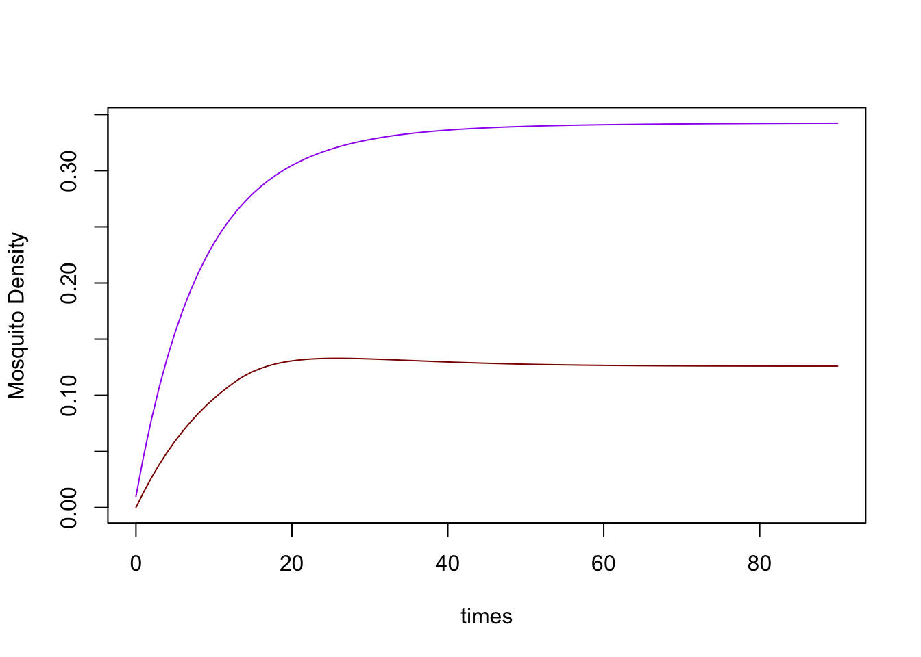

References

Macdonald G. The analysis of malaria parasite rates in infants. Tropical diseases bulletin. 1950;47: 915–938.

Macdonald G. The analysis of infection rates in diseases in which superinfection occurs. Trop Dis Bull. 1950;47: 907–915. Available: https://www.ncbi.nlm.nih.gov/pubmed/14798656

Macdonald G. Community aspects of immunity to malaria. British medical bulletin. 1951;8: 33–36.

Macdonald G. The analysis of the sporozoite rate. Trop Dis Bull. 1952;49: 569–586. Available: https://www.ncbi.nlm.nih.gov/pubmed/14958825

Macdonald G. The analysis of equilibrium in malaria. Trop Dis Bull. 1952;49: 813–829. Available: https://www.ncbi.nlm.nih.gov/pubmed/12995455

Macdonald G. The analysis of malaria epidemics. Trop Dis Bull. 1953;50: 871–889. Available: https://www.ncbi.nlm.nih.gov/pubmed/13113671

Macdonald G. A new approach to the epidemiology of malaria. Indian J Malariol. 1955;9: 261–270. Available: https://www.ncbi.nlm.nih.gov/pubmed/13306284

Macdonald G. The measurement of malaria transmission. Proceedings of the Royal Society of Medicine. 1955;48: 295–302.

Macdonald G. Epidemiological basis of malaria control. Bull World Health Organ. 1956;15: 613–626. Available: https://www.ncbi.nlm.nih.gov/pubmed/13404439

10.

Macdonald G. Theory of the eradication of malaria. Bull World Health Organ. 1956;15: 369–387. Available: https://www.ncbi.nlm.nih.gov/pubmed/13404426

11.

Malaria WEC on. Expert Committee on Malaria, Sixth Report. Athens: Geneva: Palais des Nations.; 1957. Report No.: 123. Available: https://www.cabdirect.org/cabdirect/abstract/19582900403

12.

Macdonald G. The epidemiology and control of malaria. Oxford university press; 1957. Available: https://www.cabdirect.org/cabdirect/abstract/19582900392

13.

Dobson MJ, Malowany M, Snow RW. Malaria control in East Africa: The Kampala Conference and the Pare-Taveta Scheme: A meeting of common and high ground. Parassitologia. 2000;42: 149–166. Available: http://www.ncbi.nlm.nih.gov/entrez/query.fcgi?cmd=Retrieve&db=PubMed&dopt=Citation&list_uids=11234325

14.

Fine PEM. Superinfection - a problem in formulating a problem. Tropical Diseases Bulletin. 1975;75: 475–488.

15.

Armitage P. A note on the epidemiology of malaria. Trop Dis Bull. 1953;50: 890–892.

16.

Aron JL, May RM. The population dynamics of malaria. In: Anderson RM, editor. The Population Dynamics of Infectious Diseases: Theory and Applications. Boston, MA: Springer US; 1982. pp. 139–179. Available: https://doi.org/10.1007/978-1-4899-2901-3_5