library(ramp.xds)Sharkfin Functions
A sharkfin function is a product of two sigmoidal functions – one scales up and the other scales down. The base function is:
\[\left(e^{-uk(t-D)}{1+e^{-uk(t-D)}}\right) \left(1-e^{-dk(t-L-D)}{1+e^{-dk(t-L-D)}}\right)^{pw}\]
The function is set up using makepar_F_sharkfin with the parameter names:
Dthe day when scale-up reaches 50% of its maximum value.uka shape parameter for scale-upLdays later (after D) when the scale-down reaches 50% of its maximum value.dka shape parameter for the decay phasepwa shape parameter for the decay phasemxscale to return a maximum valueNthe number of values to return
The function gets constructed in two steps. First, we configure the parameters. Next, we construct the function:
Fpar <- makepar_F_sharkfin()
F <- make_function(Fpar)
The function definition of makepar_F_sharkfin has these defaults:
makepar_F_sharkfin = function(D=100, L=180, uk = 1/7, dk=1/40,
                              pw=1, mx=1, N=1)
The function that gets returned, F, is a function of time. It a looks like a shark’s dorsal fin (or maybe an orca’s?). We have added dashed lines at \(D\) and \(L+D\)
tm <- seq(0, 500, by = 5)
plot(tm, F(tm), type = "l",
     xlab = "t - Time (in days)",
     ylab = expression(F(t)))
segments(100, 0, 100, 1, lty=2)
segments(280, 0, 280, 1, lty=2)
segments(100, .5, 280, .5, lty=2)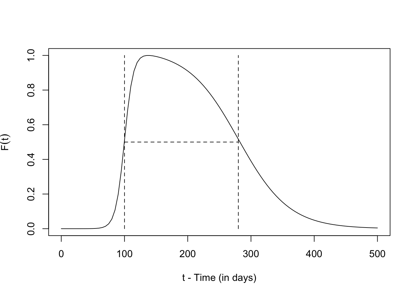
Examples
We offer the sharkfin function as-is. It’s useful, but the returned function should be checked visually or numerically before using it to ensure it has the properties desired.
library(viridisLite)
clrs <- turbo(12)
Fpar1 <- makepar_F_sharkfin(pw=2)
F1 <- make_function(Fpar1)
Fpar2 <- makepar_F_sharkfin(pw=2, L=229)
F2 <- make_function(Fpar2)plot(tm, F(tm), type = "l",
xlab = "t - Time (in days)",
ylab = expression(F(t)))
lines(tm, F1(tm), col = clrs[2])
lines(tm, F2(tm), col = clrs[4])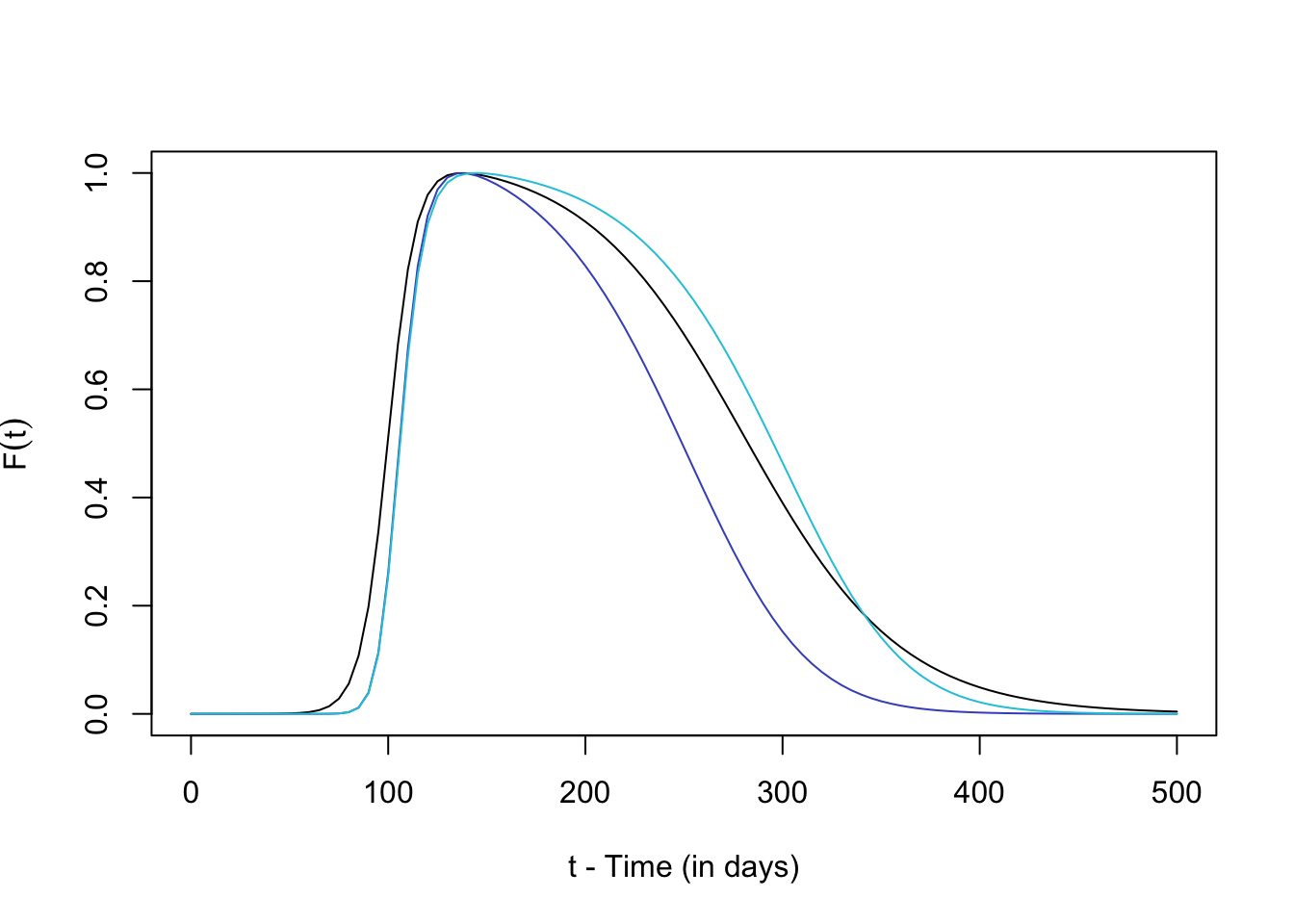
Note that if the user changes pw then it changes when the decay function reaches half its value as well as the area under the curve. This can be adjusted by changing L
integrate(F, 0, 500)$value[1] 186.2911integrate(F1, 0, 500)$value[1] 143.1431integrate(F2, 0, 500)$value[1] 186.6028