Mosquito Dispersal Kernels

Author

Affiliation

University of Washington

This vignette discusses how to set up a matrix describing mosquito dispersal.

Mosquito dispersal is understood as the outcome of flight bouts and searching for resources [1–3]. In SimBA’s patch-based framework, mosquito dispersal has two parts: emigration rates and dispersal kernels.

The mathematical framework was developed to model emigration rates in relation to the local availability of resources [4] — mosquitoes will tend to stay in patches where all the resources are readily available [3]. Emigration and the hazards associated with dispersal are probably an important source of mosquito mortality [5]. Knowing that a mosquito has left a patch is one thing, but the models must also say where they land, which can be affected by specific features on a landscape [6–10]. If mosquito dispersal is the result of a flight bouts, where the direction and distances traveled are affected by wind [2,3,11–13], then a mosquito leaving a patch could end up anywhere, not just in a neighboring patch. This calls for a general framework to model dispersal among patches. The framework thus handles mosquito dispersal in two parts: emigration and emigration loss are one part; and the destinations of emigrating mosquitoes that survive is the other.

This vignette describes mosquito dispersal kernels — a matrix describing where the surviving emigrants end up. Emigration rates and population loss associated with dispersal are handled separately (see Mosquito Demography), so by convention, each column sums up to zero.

In ramp.xds, a mosquito dispersal kernel can be configured as part of basic setup, or it can be changed later using setup_K_matrix, which handles setup for models with minimal ecology as well as behavioral state models.

This vignette covers:

Dispersal Kernels — the standard implementation of dispersal kernels across all MY modules
setup_K_matrix() — a discussion of setup_K_matrix() and its methods:
- matrix — set up \(K\) by passing an \(N_p \times N_p\) matrix with the proper form
- herethere — disperse evenly to all other patches
- xy — use the \(x,y\) locations and a spatial kernel
- zero — set the matrix to all zeros
- N — for behavioral state models, set up multiple kernels
xds_setup() — how xds_setup() handles dispersal kernels
Examples

Emigration & Loss

We let \(\sigma\) denote the patch emigration rate. The parameter \(\mu\) describes population loss that is conditioned on emigration from a patch: a fraction \(\mu\) never reaches another patch. If \(g\) is the mortality rate (in each patch), then mortality and migration terms are summarized by a single matrix, \(\Omega,\) called the mosquito demographic matrix

\[\Omega = \mbox{diag}\left(g + \sigma \mu\right) - K \cdot \mbox{diag}\left(\sigma \left(1-\mu\right) \right)\] The dispersal kernel \(K\) is called the dispersal kernel or the K_matrix. For more information, see Mosquito Demography.

Dispersal Kernels

Let \(k_{i,j}\) describe the fraction of mosquitoes emigrating from each patch that land on another patch: \({k}_{i,j} (t) \in K(t)\) is the fraction of mosquitoes leaving patch \(j\) that end up in patch \(i\). Each column in the matrix describes mosquitoes leaving from \(j.\) The columns of \(K\) sum to 0.

\[\begin{equation} K = \left[ \begin{array}{ccccc} j=1&j=2&j=3&\cdots&j=p \\ \boxed{ \begin{array}{c} -1 \\ {k}_{2,1} \\ {k}_{3,1} \\ \vdots \\ {k}_{p,1} \\ \end{array}} & \boxed{ \begin{array}{c} {k}_{1,2} \\ -1 \\ {k}_{3,2} \\ \vdots \\ {k}_{p,2} \\ \end{array}} & \boxed{ \begin{array}{c} {k}_{1,3} \\ {k}_{3,2} \\ -1 \\ \vdots \\ {k}_{p,3} \\ \end{array}} & \boxed{ \begin{array}{c} \cdots \\ \cdots \\ \cdots \\ \ddots \\ \cdots \end{array}} & \boxed{ \begin{array}{c} {k}_{1,p} \\ {k}_{2,p} \\ {k}_{3,p} \\ \vdots \\ -1 \\ \end{array}} \end{array} \right] \end{equation}\]

Behavioral state models often have two or more dispersal matrices.

`setup_K_matrix`

library(ramp.xds)

The function used to configure the dispersal kernels is called setup_K_matrix. The function call is:

setup_K_matrix(name, xds_obj, options=list(), s=1)

Inline help is available:

?xds_info_mosquito_dispersal
?setup_K_matrix

The function setup_K_matrix dispatches on options but before function is dispatched, a block of code is run that makes it possible to pass arguments in several ways.

but class(name) is checked and changed before the function call:

The function was designed to be called by passing a string called name, the name of the S3 method:
- if name is a string, then class(options) <- 'name'
- options is a named list with arguments for setup_K_matrix.name
Matrix
- if name is a matrix, then class(options) <- 'as_matrix'
- it is equivalent to calling `setup_K_matrix(“as_matrix”, options = )
if name is a list with an item called name the function dispatches on setup_K_matrix.list.

`as_matrix`

The as_matrix option makes it possible to build a matrix using any method and use it as a K_matrix, so long as it has the right form. The matrix is checked by check_K_matrix

?check_K_matrix

my_M = matrix(c(-1, .97, .03, 
             .95, -1, .05, 
             0.02, .98, -1), 3, 3)
my_M

      [,1]  [,2]  [,3]
[1,] -1.00  0.95  0.02
[2,]  0.97 -1.00  0.98
[3,]  0.03  0.05 -1.00

check_K_matrix(my_M, 3)

After setting up a model, the matrix can be set up in two ways.

model <- xds_setup(nPatches = 3)

The call to setup_K_matrix using the standard syntax is:

model1 <- setup_K_matrix("as_matrix", model, list(K_matrix=my_M))
get_K_matrix(model1)

      [,1]  [,2]  [,3]
[1,] -1.00  0.95  0.02
[2,]  0.97 -1.00  0.98
[3,]  0.03  0.05 -1.00

An easier way is to pass the matrix instead of the name:

model2 <- setup_K_matrix(my_M, model)
get_K_matrix(model2)

      [,1]  [,2]  [,3]
[1,] -1.00  0.95  0.02
[2,]  0.97 -1.00  0.98
[3,]  0.03  0.05 -1.00

`herethere`

If name = "herethere" then the fraction moving to every other patch is equal. There are no parameters:

model <- setup_K_matrix("herethere", model)
get_K_matrix(model)

     [,1] [,2] [,3]
[1,] -1.0  0.5  0.5
[2,]  0.5 -1.0  0.5
[3,]  0.5  0.5 -1.0

`xy`

The setup_timspent.xy option grabs the residence vector and then calls make_K_matrix_xy with options:

xy — the \(x\) and \(y\) coordinates of each patch
F_K — a function to weight relative travel among patches by distance with the form \[F_K(d, V)\]
V — a set of variables to pass to \(F_K\)

For example, we generate 10 random points:

nXY=20
model_xy = xds_setup(nPatches=nXY)

xy = data.frame(x=runif(nXY, -5, 5), y=runif(nXY, -5, 5))

We construct a function: \[F_K(d,V) = e^{-(d-3)^2}.\]

FdV = function(d, V=list()){exp(-(d-3)^2)}

K_xy <- make_K_matrix_xy(xy, FdV)

library(ramp.qa)
plot_kernel_graph(K_xy, xy, mn=0.01, clrs = viridisLite::turbo(10),
                        arr.pos=0.7, scl=2)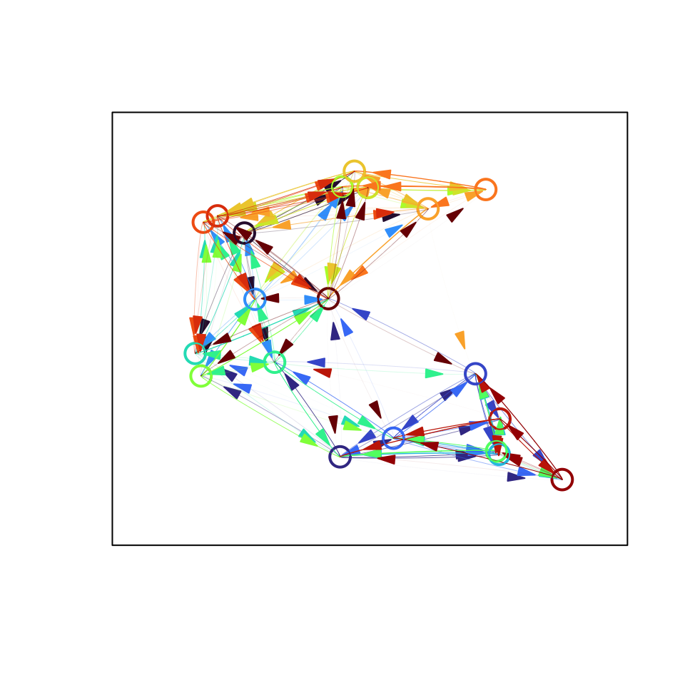

This sets up the model:

model_xy = setup_K_matrix("xy", model_xy, 
                          list(xy=xy, F_K=FdV, V=list()))

Behavioral State Models

The dispersal kernels for behavioral state models are the result of searching for different resources. For basic ecology models, the dispersal kernel is called K_matrix, but behavioral state models can have two or more kernels, each with different names.

To handle this, the functions get_K_matrix and change_K_matrix have an extra argument which_K. By default, for basic ecology, the default is set to “K” and it can be ignored. It can not be ignored when working with behavioral state models.

The behavioral state models are in ramp.library so we load it.

library(ramp.library)

The BQ module is a behavioral state module. We’ll set one up to work with:

modBQ <- xds_setup(MYname = "BQ", nPatches=3)

To look at the \(K_b\) matrix (for blood searching), we use get_K_matrix with the second argument, Kb

get_K_matrix(modBQ, "Kb")

     [,1] [,2] [,3]
[1,]    0    0    0
[2,]    0    0    0
[3,]    0    0    0

We can call setup_K_matrix to change it, but we must add which_K = "Kb" to the options list:

modBQ <- setup_K_matrix("herethere", modBQ, options=list(which_K = "Kb"))
get_K_matrix(modBQ, "Kb")

     [,1] [,2] [,3]
[1,] -1.0  0.5  0.5
[2,]  0.5 -1.0  0.5
[3,]  0.5  0.5 -1.0

A method for setup_K_matrix was written for behavioral state models. The method name is “N”, and the argument must say now many kernels it will be setting up: \(N=2\). The options must also have an argument called opts which is a list of length \(N\): each one describes how to set up the kernel. For example:

Kopts = list(name = "N", N=2, opts = list()) 
Kopts$opts[[1]] = list(name = "herethere", which_K = "Kb")
Kopts$opts[[2]] = list(name = "herethere", which_K = "Kq")

Now, we can set up a model and then modify both kernels at the same time. After basic setup, the kernels are both set to \(0\) matrices.

modBQ4 <- xds_setup(MYname = "BQ", nPatches=4)
get_K_matrix(modBQ4, "Kq")

     [,1] [,2] [,3] [,4]
[1,]    0    0    0    0
[2,]    0    0    0    0
[3,]    0    0    0    0
[4,]    0    0    0    0

Now, we pass the options, and we get:

modBQ4 <- setup_K_matrix("N", modBQ4, Kopts)
get_K_matrix(modBQ4, "Kq")

           [,1]       [,2]       [,3]       [,4]
[1,] -1.0000000  0.3333333  0.3333333  0.3333333
[2,]  0.3333333 -1.0000000  0.3333333  0.3333333
[3,]  0.3333333  0.3333333 -1.0000000  0.3333333
[4,]  0.3333333  0.3333333  0.3333333 -1.0000000

get_K_matrix(modBQ4, "Kb")

           [,1]       [,2]       [,3]       [,4]
[1,] -1.0000000  0.3333333  0.3333333  0.3333333
[2,]  0.3333333 -1.0000000  0.3333333  0.3333333
[3,]  0.3333333  0.3333333 -1.0000000  0.3333333
[4,]  0.3333333  0.3333333  0.3333333 -1.0000000

Basic Setup

The time spent matrix can be configured in basic setup.

Defaults

The default setting for xds_setup is that mosquitoes don’t move. If \(N_p=1\) then the time spent matrix for one patch is:

model <- xds_setup()
get_K_matrix(model)

     [,1]
[1,]    0

For multiple strata:

model <- xds_setup(nPatches=3)
get_K_matrix(model)

     [,1] [,2] [,3]
[1,]    0    0    0
[2,]    0    0    0
[3,]    0    0    0

`Koptions`

At setup, a parameter list called Koptions can be passed that calls setup_K_matrix. Any list of options that would set up a kernel using setup_K_matrix will work here. For example:

model <- xds_setup(nPatches=3, Koptions = list(name="herethere"))
get_K_matrix(model)

     [,1] [,2] [,3]
[1,] -1.0  0.5  0.5
[2,]  0.5 -1.0  0.5
[3,]  0.5  0.5 -1.0

Note that for behavioral state models, we could also pass Kopts to xds_setup

modBQ5 <- xds_setup(MYname = "BQ", nPatches=5, Koptions=Kopts)
get_K_matrix(modBQ5, "Kb")

      [,1]  [,2]  [,3]  [,4]  [,5]
[1,] -1.00  0.25  0.25  0.25  0.25
[2,]  0.25 -1.00  0.25  0.25  0.25
[3,]  0.25  0.25 -1.00  0.25  0.25
[4,]  0.25  0.25  0.25 -1.00  0.25
[5,]  0.25  0.25  0.25  0.25 -1.00

Examples

A Spatial Kernel

Service MW. Mosquito (Diptera: Culicidae) dispersal–the long and short of it. J Med Entomol. 1997;34: 579–588. doi:10.1093/jmedent/34.6.579

Wu SL, Sánchez C HM, Henry JM, Citron DT, Zhang Q, Compton K, et al. Vector bionomics and vectorial capacity as emergent properties of mosquito behaviors and ecology. PLoS Comput Biol. 2020;16: e1007446. doi:10.1371/journal.pcbi.1007446

Sánchez C HM, Wu SL, Henry JM, Guerra CA, Galick DS, Garcia GA, et al. Mosquito dispersal in context. PLOS Complex Systems. 2026;3: e0000108. doi:10.1371/journal.pcsy.0000108

Wu SL, Henry JM, Citron DT, Ssebuliba DM, Nsumba JN, C HMS, et al. Spatial dynamics of malaria transmission. PLoS Computational Biology. 2023;19: e1010684. doi:10.1371/journal.pcbi.1010684

Saul A. Zooprophylaxis or zoopotentiation: The outcome of introducing animals on vector transmission is highly dependent on the mosquito mortality while searching. Malaria Journal. 2003;2: 32. doi:10.1186/1475-2875-2-32

Bidlingmayer WL, Franklin BP, Jennings AM, Cody EF. Mosquito flight paths in relation to the environment. Influence of blood meals, ovarian stage and parity. Ann Entomol Soc Am. 1974;67: 919–927. Available: http://www.ingentaconnect.com/content/esa/aesa/1974/00000067/00000006/art00021

Bidlingmayer WL, Hem DG. Mosquito (Dipteral Culicidae) flight behaviour near conspicuous objects. Bulletin of Entomological Research. 1979;69: 691–700. doi:10.1017/S0007485300020228

Bidlingmayer WL, Hem DG. Mosquito flight paths in relation to the environment: Effect of the forest edge upon trap catches in the field. Mosq News. 1981;41. Available: http://agris.fao.org/agris-search/search/display.do?f=2012/OV/OV201202911002911.xml;US19820737712

Bidlingmayer WL. The measurement of adult mosquito population changes–some considerations. J Am Mosq Control Assoc. 1985;1: 328–348. Available: http://eutils.ncbi.nlm.nih.gov/entrez/eutils/elink.fcgi?dbfrom=pubmed&id=2906674&retmode=ref&cmd=prlinks

10.

Lutambi AM, Penny MA, Smith TA, Chitnis N. Mathematical modelling of mosquito dispersal in a heterogeneous environment. Math Biosci. 2013;241: 198–216. doi:10.1016/j.mbs.2012.11.013

11.

Bidlingmayer WL, Evans DG, Hansen CH. Preliminary study of the effects of wind velocities and wind shadows upon suction trap catches of mosquitoes (Diptera: Culicidae). J Med Entomol. 1985;22: 295–302. Available: http://eutils.ncbi.nlm.nih.gov/entrez/eutils/elink.fcgi?dbfrom=pubmed&id=2861290&retmode=ref&cmd=prlinks

12.

Midega JT, Smith DL, Olotu A, Mwangangi JM, Nzovu JG, Wambua J, et al. Wind direction and proximity to larval sites determines malaria risk in Kilifi District in Kenya. Nat Commun. 2012;3: 674. doi:10.1038/ncomms1672

13.

Perkins TA, Scott TW, Le Menach A, Smith DL. Heterogeneity, mixing, and the spatial scales of mosquito-borne pathogen transmission. PLoS Comput Biol. 2013;9: e1003327.