Trace Functions

Configuring

library(ramp.xds)

We have been using the term trace function to describe a function that sets the value of the quantity that is passed from each component, in place of a fully defined dynamical component. To build in some flexibility in a way that is easy for users to work with, all trace functions are colled in the same way.

When the class of any module is set to trivial, the quantities passed from that module are all called in the same way:

\[s \times F_S(t) \times F_T(t)\]

where:

\(s\) is a scaling parameter;
\(F_S(t)\) is a seasonal pattern;
\(F_T(t)\) defines a temporal trend;

Scaling

The name of the scaling parameter depends on context:

Lambda or \(\Lambda\) for the emergence rate, passed from the L component when it is trivial. The setup function is

?make_Lpar_trivial

fqZ or \(fqZ\) (from F_fqZ) for the net human blood feeding rate, per patch, passed from the MYZ component when it is ’trivial` and X is non-trivial. The setup function is

?make_MYZpar_trivial

eggs (from F_eggs) for the egg laying rate in each patch, net human blood feeding rate, per patch, passed from the MYZ component when it is ’trivial` and L is non-trivial. The setup function is

?make_MYZpar_trivial

kappa (from F_X) to compute net infectiousness, or \(\kappa\) passed from the X component when it is ’trivial` and MYZ is non-trivial. The setup function is

?make_Xpar_trivial

Seasonality

To configure the seasonality function, either define a function and pass it as F_season or pass season_par in the options, with parameters called by the xds utility make_function()

Lo = list(season_par = makepar_F_sin()) 
sin_mod <- xds_setup(Lopts = Lo)

Now, the function can be evaluated:

tt <- 0:365
Fs <- sin_mod$Lpar[[1]]$F_season
plot(tt, Fs(tt), type ="l")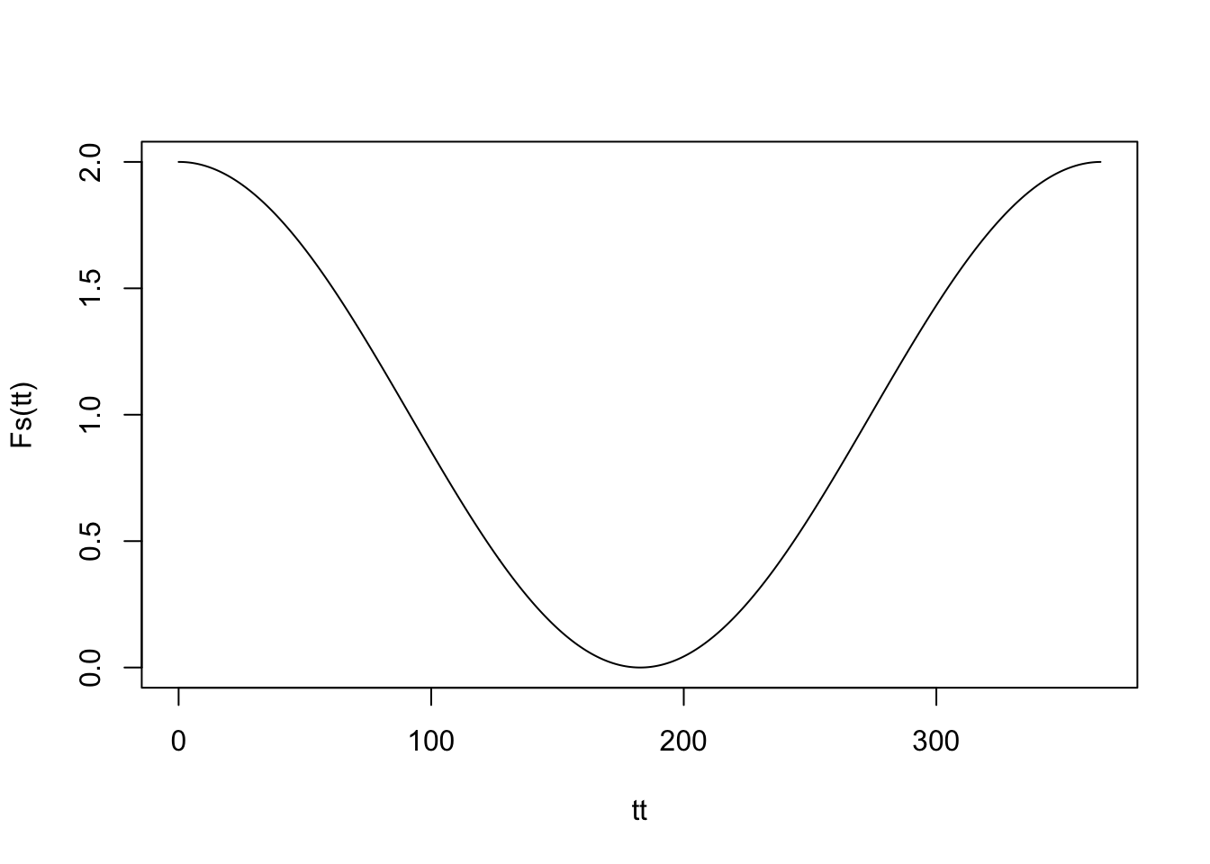

As a side note, if you use <- instead of = when you define the list, the damn thing doesn’t work. Note that the phase parameter is defined:

sin_mod$Lpar[[1]]$season_par$phase

[1] 0

but this doesn’t set anything:

Lo = list(season_par <- makepar_F_sin()) 
sin_mod1 <- xds_setup(Lopts = Lo)
sin_mod1$Lpar[[1]]$season_par

list()

Trend

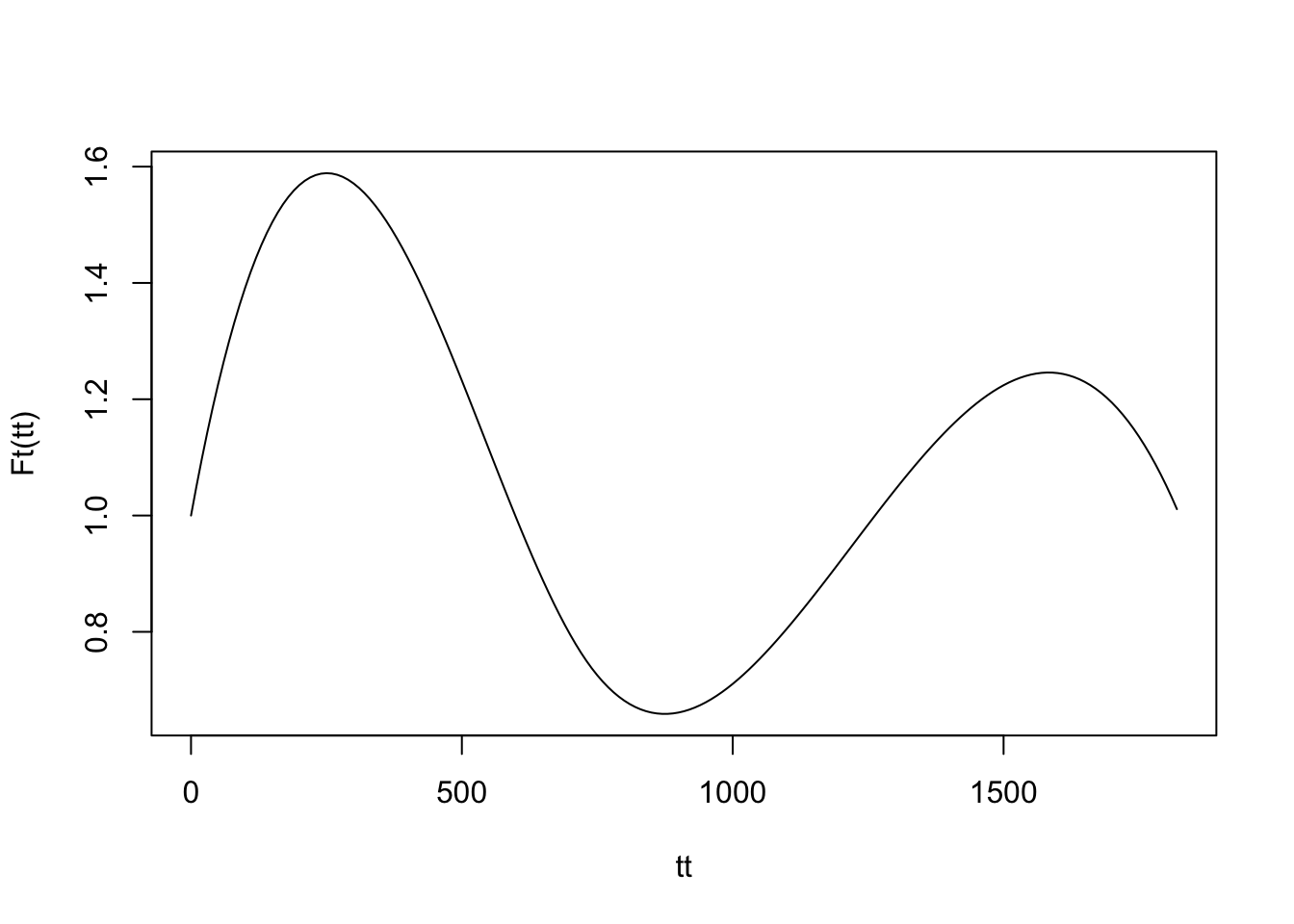
To configure a trend function, either define a function and pass it as F_trend or pass trend_par in the options, with parameters called by the xds utility make_function()

Lo = list(trend_par = makepar_F_spline(tt = c(0:5)*365, yy= c(1, 1.5, .75, .8, 1.2, 1))) 
trend_mod <- xds_setup(Lopts = Lo)

Now, the function can be evaluated:

tt <- seq(0, 5*365, by = 10)
Ft <- trend_mod$Lpar[[1]]$F_trend
plot(tt, Ft(tt), type ="l")