library(ramp.xds)
library(ramp.library)Solve a Model
SimBA Basics: Vignette 3
This vignette assumes:
you know about mathematical models for malaria;
you know how to use R and RStudio;
you have installed the software. This loads it:
- you know how to build a model. This builds the default model:
model <- xds_setup()xds_solve
The object we called model defines a dynamical system. To solve model, the default call is:
model <- xds_solve(model)Solutions
The solutions are parsed and attached as named lists to model$outputs. The solutions can be retrieved using the functions get_XH_out or get_MY_out or get_L_out.
Time
Optional arguments can be passed to xds_solve to specify the time points to evaluate the dependent variables:
If the argument
timesis passed (i.e., if it is not null), then the model assumes the initial values for the dependent variables correspond to the first value intimesand it returns the values of the variables at the other values in the vector.Otherwise, a user may pass values for
Tmaxanddt. The values of the variables are returned \(t=\)seq(0, Tmax, by=dt). By default,Tmax=365anddt=1.
Values of time (the dependent variable) are stored as model$outputs$time. This checks what we’ve just said:
sum((c(0:365) - model$outputs$time)^2)[1] 0To learn more, read on.
Solving
What does it mean to solve a system of differential equations?
Solving a system of differential equations means computing solutions to the initial value problem: given the values of state of the system at a single point in time, what are the values of dependent variables at other points in time? The values of these dependent variables are called the trajectories or orbits.
In ramp.xds, the function xds_solve solves the initial value problem. attaches the orbits to the xds object, and returns it. For differential equations, the solutions are generated by a call to either ode or dede in an R package called deSolve that numerically solves the equations.
The solutions can be retrieved using functions caled get_XH_out or get_MY_out. In the next vignette, we describes some built-in functions to make visualization easier. Here, we use these functions to plot some outputs:
names(get_XH_out(model))[1] "S" "I" "H" "eir" "foi" "ni" "true_pr"
[8] "time" This plots the number of infected humans over time (in days):
with(get_XH_out(model), plot(time, I, type = "l",
                             main = "Humans", ylab = "I - Number Infected"))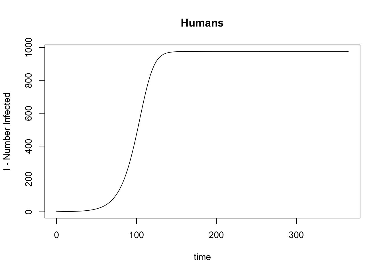
names(get_MY_out(model)) [1] "M" "P" "Y" "Z" "y" "z" "parous" "fqM"
[9] "G" "Lambda" "kappa" "time" with(get_MY_out(model), plot(time, Z, type = "l",
main = "Mosquitoes", ylab = "Z - Number Infectious"))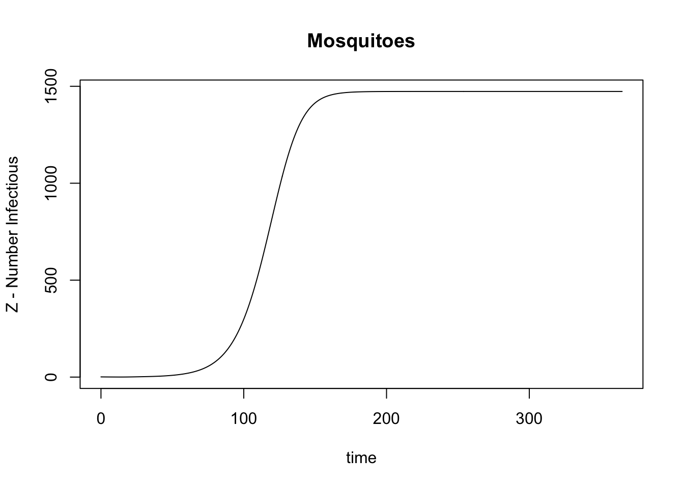
Outputs
We can see how it stores the outputs:
deoutis the matrix returned bydeSolvetimeis the value of the dependent variableslast_yis the final state of the systemorbitsholds the solutions
names(model$outputs)[1] "deout" "time" "last_y" "orbits"The outputs are parsed by name and stored separately by component:
names(model$outputs$orbits)[1] "L" "MY" "XH"We can see what it returns by asking for names. (Since there might be more than one host species, we must specify the first). For the XH component, it returns the variables and some terms:
names(model$outputs$orbits$XH[[1]])[1] "S" "I" "H" "eir" "foi" "ni" "true_pr"Similarly, we can look at the variables describing the adult mosquito populations and some terms:
names(model$outputs$orbits$MY[[1]]) [1] "M" "P" "Y" "Z" "y" "z" "parous" "fqM"
[9] "G" "Lambda" "kappa" There are functions to make visualization easier (see Visualization), but it’s pretty easy to
with(model$outputs, plot(time, orbits$XH[[1]]$I, type = "l", ylab = "I"))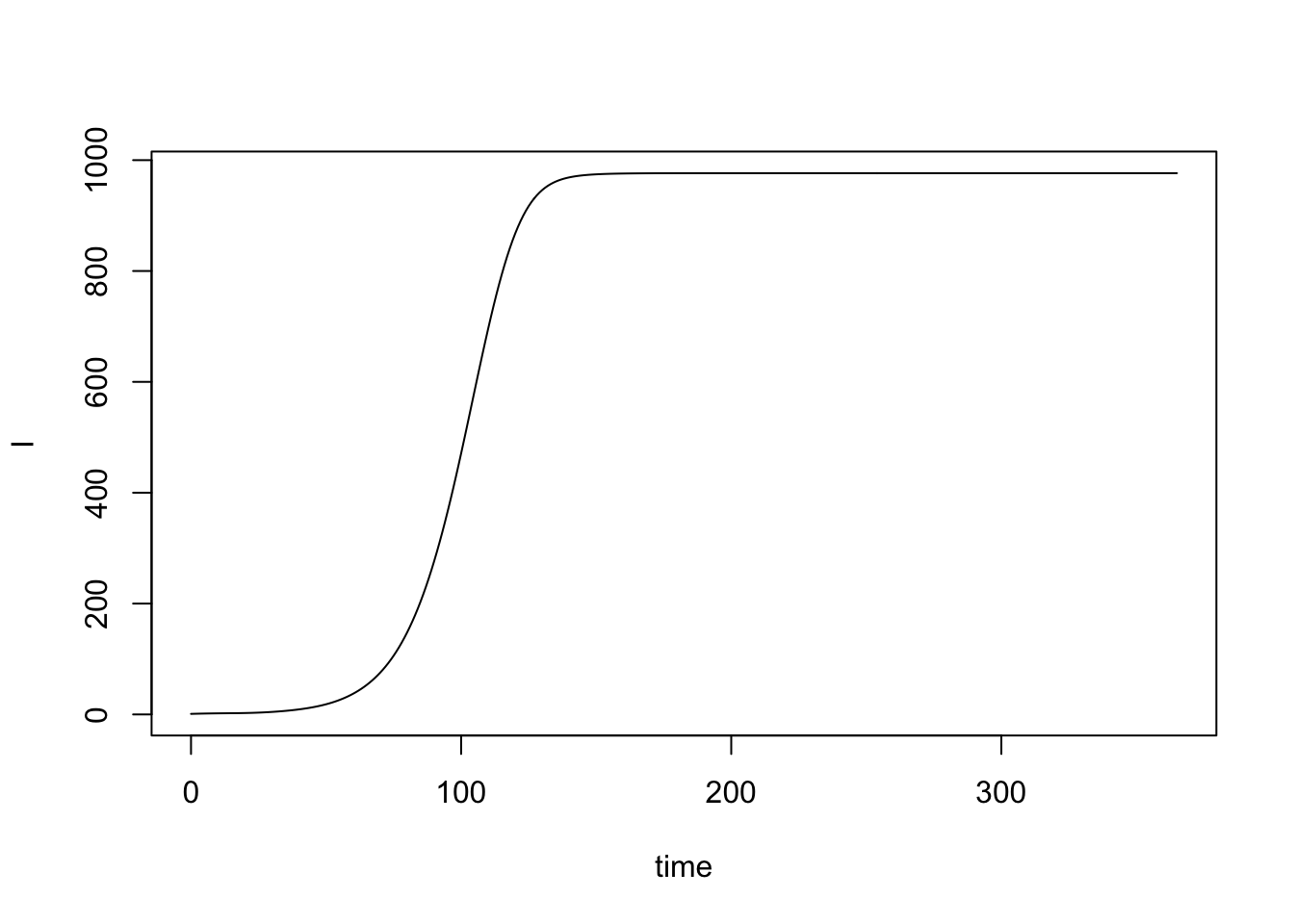
The parts of a model
To get a little more specific, every dynamical system includes:
An independent variable: in these equations, the independent variable is time.
One or more dependent variables
Initial values of the dependent variables
A system of equations or functions that compute the derivatives (for differential equations) or update the values of the variables (for discrete time systems)
A fully defined set of parameters
What are they?
model[1] HUMAN / HOST
[1] # Species: 1
[1]
[1] X Module: SIS
[1] # Strata: 1
[1]
[1] VECTORS
[1] # Species: 1
[1]
[1] MY Module: macdonald
[1] # Patches: 1
[1]
[1] L Module: trivial
[1] # Habitats: 1 the XH component – infection and immune dynamics and demography human or host populations – is the
SISmodule, an SIS compartment modelthe MY component is the
macdonaldmodule: the infection dynamics a delayed SI compartmental modelthe L component is defined by the
trivialmodule: it does not have any variables. In this case, the emergence rate of adult mosquitoes is a default function with default values.