Chapter 16 Trees and Forests
We assume you have loaded the following packages:
Below we load more as we introduce more.
16.1 Trees and forests in sklearn
sklearn library provides a number of decision-tree related methods.
The central ones we discuss here are DecisionTreeRegression and
DecisionTreeClassifier. The former is designed for regression tasks
(continuous target) and the latter for categorization tasks
(categorical target). The usage of both is similar to the other
supervised ML models in sklearn, such as linear regression and
logistic regression (see Sections
10.2.2 and
11.2.2).
As in case of other sklearn regression models, we have to proceed in following steps:
- Create the design matrix \(\mathsf{X}\) and the target vector \(\boldsymbol{y}\).
- Set up the model, we call it m. For decision trees you may want to set various parameters (see below), unlike in case of linear regression.
- Fit the model using the
.fit(X, y)-method. - Use the fitted model to compute accuracy or \(R^2\) (the
.score()method), or use it for predictions.
Obviously, you may want to use other relevant tools, such as training-validation split when doing these tasks.
The DecisionTreeRegression and
DecisionTreeClassifier allow for a large number of options. The
most relevant are
- max_depth: maximum depth of the tree to build
- min_samples_split: minimum node size to be considered for splitting
See more in the sklearn documentation.
Besides decision trees, the book also provides examples of bagging
(BaggingClassifier(), see Section 16.4),
random forests (RandomForestClassifier(), see Section
16.5,
and Adaboost (AdaBoostClassifier(), see Section 16.6).
Below, we demonstrate the basic usage and visualization through different examples, first using regression trees and thereafter classification trees.
16.2 Regression Trees
Below is an example how to use decision trees for regression tasks. We focus on a 1-D case as this is easy to visualize. We use Boston housing data to predict the house prices based on the number of rooms.
First, we load data and create the matrices:
In order to use regression trees, we need to import the function, set up the model, and fit it. Below, we specify the maximum depth 2, again for easier visualization:
## /usr/lib/python3/dist-packages/scipy/__init__.py:146: UserWarning: A NumPy version >=1.17.3 and <1.25.0 is required for this version of SciPy (detected version 1.26.4
##   warnings.warn(f"A NumPy version >={np_minversion} and <{np_maxversion}"
m = DecisionTreeRegressor(max_depth=2)
_t = m.fit(X, y)
m.score(X, y) # on training data, may not be reliable## 0.5828967342544766## /home/siim/.local/lib/python3.10/site-packages/sklearn/base.py:493: UserWarning: X does not have valid feature names, but DecisionTreeRegressor was fitted with feature names
## warnings.warn(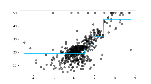
plot of chunk boston-2
Boston housing data, including the relationship as predicted by the depth-2 tree (the light-blue zig-zag line).
We can plot it using the following code:
xx = np.linspace(X.rm.min(), X.rm.max(),
                 300).reshape((-1,1))
# reshape to 2-D
yhat = m.predict(xx)
_ = plt.scatter(X.rm, y,
                color = "black",
                alpha=0.5)
_ = plt.plot(xx, yhat,
             color = "deepskyblue")
plt.show()
We begin by creating a equally-spaced sequence of 300 points that stretches the same range as the variable rm. We need to reshape it into a matrix, otherwise sklearn cannot use it for predictions. Thereafter we predict the values using all these datapoints. As you can see, the predicted values form a piecewise-constant curve (light-blue on the figure), this is how rectangular regions look in one dimension.
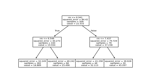
plot of chunk boston-tree-plot
The tree above, as visualized by plot_tree().
If you want to visualize the tree structure, you can use plot_tree()
function from sklearn.tree:
This is is simple and often good enough, but it may be hard to fit into an html document as one can see here.

The tree above, as visualized by graphviz package.
More complex visualizations can be done with graphviz package:
import graphviz
from sklearn.tree import export_graphviz

dot = export_graphviz(m, out_file=None,
                      feature_names=X.columns,
                      filled=True)
graph = graphviz.Source(dot, format="svg")
_ = graph.render("boston-tree-graphviz",
                 directory=".fig")
Here one has to start by creating a dot object that describes the structure of the tree. Afterward it is sourced as graph, and finally rendered. Here it is rendered as a svg file, displayed in the browser at right. Graphviz package has many more options, consult the documentation for details.
Exercise 16.1 Use Boston Housing data.
- Estimate the median price (medv) as a function of average number of
rooms (rm) and age (age) using regression trees. Use
max_depth=2as above. - Compute \(R^2\) on training data. Did it improve over what we found above?
- Visualize the corresponding regression tree using
plot_treeor graphviz. How does the tree differ from the only-rm tree above? - Now include all the features in your model (all columns, except medv) and repeat the above: compute \(R^2\) and visualize the tree. Does adding more features change the tree in any significant way?
See The Solution
16.3 Classification Trees
This section demonstrates the usage of classification trees using Yin-Yang data (see Section 23.5).
16.3.1 Doing classification trees in sklearn
First load the dataset. For a refresher, it contains three variables, x, y, and c; the first two are coordinates on \(x-y\)-plane, and the latter (0 or 1) is color. Load it and have a look:
##           x         y  c
## 0 -1.627663  0.583590  0
## 1  0.624083 -0.113418  0
## 2 -0.687947  1.743150  1
Decision trees in sklearn work in a similar fashion as other sklearn categorization models. In particualr, you need to import the method (DecisionTreeClassifier), create the model, fit the model, and use it for any kind of predictive analysis. For fitting, we need the design matrix X and the outcome vector y. sklearn can typically handle both data frames and matrices, but the decision boundary code below assumes we use matrices. So we ensure they are matrices:
from sklearn.tree import DecisionTreeClassifier

y = yy.c.values  # .values converst to numpy vector
X = yy[["x", "y"]].values  # conver to numpy matrix

m = DecisionTreeClassifier()
_t = m.fit(X, y)
m.score(X, y)  # accuracy on training data
## 1.0Here we followed the standard sklearn’s approach: fit the model, and
compute accuracy using .score(). By default, the trees overfit
and hence we get accuracy 1 on training data.
16.3.2 Decision boundary
One of the most instructive ways to understand the models it to plot their decision boundary. This is only possible for 2-D models (features form a 2-D space), in 1-D case it is just a set of points, in 3-D case it is complicated, and in case of more features, it is impossible.
Here is a function that makes such a plot. It has 4 arguments: a fitted model, design matrix X, outcome vector y, and number of grid points. This version assumes that X and y are numpy matrices, not pandas’ objects. The actual values are used for a) finding the extent of data to be plotted; and b) to be added to the actual plot, for visual guidance.
def DBPlot(m, X, y, nGrid = 100):
    ## find the extent of the features
    ## and add 'padding', here "1" to it.  Adjust as needed!
    x1_min, x1_max = X[:, 0].min() - 1, X[:, 0].max() + 1
            # note: indexing assumes X is a np.array!
    x2_min, x2_max = X[:, 1].min() - 1, X[:, 1].max() + 1
    ## make a dense grid (nGrid x nGrid) in this extent
    xx1, xx2 = np.meshgrid(np.linspace(x1_min, x1_max, nGrid),
                           np.linspace(x2_min, x2_max, nGrid))
    ## Convert two grids into two columns
    XX = np.column_stack((xx1.ravel(), xx2.ravel()))
    ## predict on the grid
    hatyy = m.predict(XX).reshape(xx1.shape)
    plt.figure(figsize=(8,8))
    ## show the predictions as an semi-transparent image
    _ = plt.imshow(hatyy, extent=(x1_min, x1_max, x2_min, x2_max),
                   aspect="auto",
                   interpolation='none', origin='lower',
                   alpha=0.3)
    ## add the actual data points on the image
    plt.scatter(X[:,0], X[:,1], c=y, s=30, edgecolors='k')
    plt.xlim(x1_min, x1_max)
    plt.ylim(x2_min, x2_max)
    plt.show()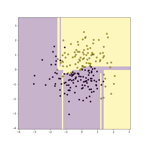
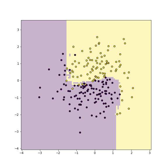
plot of chunk dbplot-yy
Now we can plot the decision boundary of the fitted tree model as
This shows which areas are predicted as purple, and which ones as gold. The figure shows pretty clearly that the current tree splits the feature space into too detailed rectangles–it carves out single rectangles for individual purple and yellow dots. This is how it achieves the perfect accuracy, but as we only work on training data, it is obviously overfitting.
16.4 Bagging
Bagging involves bootstrapping from the original data many times, and each time fitting a different decision tree. Final decision will be done by all these trees by majority voting.
The main workhorse isBaggingClassifier(). Its most important
argument is n_estimators, how many different trees to build.

16.5 Random Forests
Random forests are similar to bagging, but besides each time randomly bootstrapping from data, it also pics a random subset of features. In practice, random forests tend to work much better than bagging.
The main workhorse isRandomForestClassifier() where the argument
n_estimators tells how many different trees to build.
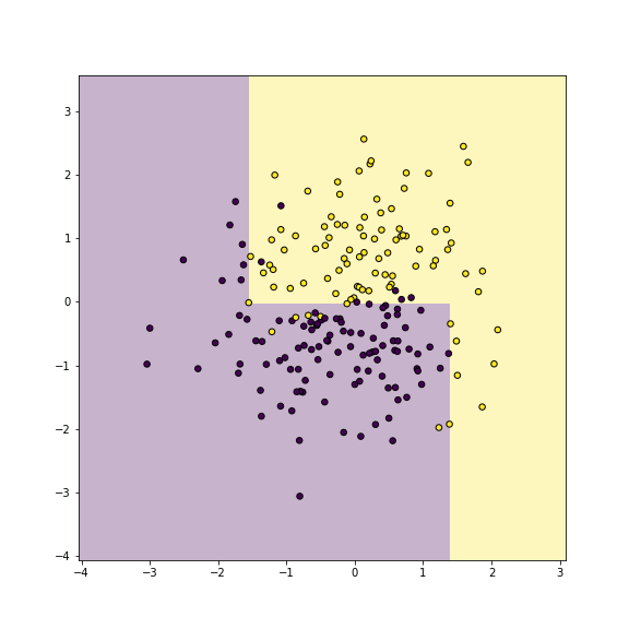
plot of chunk unnamed-chunk-14
Yin-yang data using random forest classifier. Training accuracy is 1.
from sklearn.ensemble import\
    RandomForestClassifier

m = RandomForestClassifier(
    n_estimators = 100)
_t = m.fit(X, y)
On these data, there is not much of a difference between bagging and random forests, because there are only two features.
16.6 Boosting
Boosting also involves creating a number of simple trees. Unlike bagging and random forests, it keeps increasing the weights on misclassified cases until it achieves good results. Boosting tends to work better than both bagging and random forests.
The main workhorse isAdaBoostClassifier() where the argument
n_estimators tells how many different trees to build.
## /home/siim/.local/lib/python3.10/site-packages/sklearn/ensemble/_weight_boosting.py:527: FutureWarning: The SAMME.R algorithm (the default) is deprecated and will be removed in 1.6. Use the SAMME algorithm to circumvent this warning.
##   warnings.warn(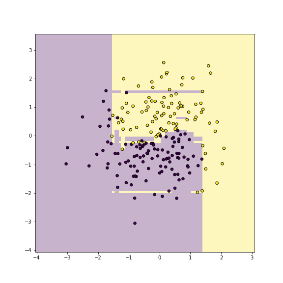
plot of chunk unnamed-chunk-15
Yin-yang data using Ada-boost classifier. Training accuracy is 1.