Chapter 12 Predictions and Model Goodness
Predictions have a wide range of applications, and in many cases we are not interested in inference, i.e. we are not interested in the parameter values and their interpretation. The python libraries we consider here, statsmodels and sklearn offer easy approaches for predictions, but we start with manual computation, just to make it clear how the models actually work. We spend more time on linear regression, in case of logistic regression we stress more the different types of predictions–probabilities and categories.
Libraries we use in this section:
import numpy as np
import pandas as pd
import matplotlib.pyplot as plt
import statsmodels.formula.api as smf
We also import functions from sklearn library as we need.
12.1 Predicting with Linear Regression Models
Linear regression is designed for continuous numeric outcome variables, such as physical dimensions or income. Below we demonstrate three ways to compute the related predictions: manually, using both scalar and matrix algebra, by using statsmodels, and finally with sklearn library.
12.1.1 Predicting linear regression outcomes manually
We provide two examples here. First we do a simple regression example using ordinary scalar algebra where we predict the distance to galaxies on hubble data, and thereafter we show how one can predict multiple regression results with matrix algebra.
12.1.1.1 Simple regression without linear algebra
We start with a simple regression example where the task is to predict distance of galaxies by their radial velocity using Hubble data. First we estimate a model \[\begin{equation} \text{R}_i = \beta_0 + \beta_1 \cdot \text{v}_i + \epsilon_i, \end{equation}\] where \(R\) is distance (in Mpc) and \(v\) is radial velocity of galaxy \(i\):
##        object  ms      R    v   mt    Mt     D  Rmodern  vModern
## 0      S.Mag.  ..  0.032  170  1.5 -16.0  0.03  0.06170    158.1
## 1      L.Mag.  ..  0.030  290  0.5 -17.2  0.03  0.04997    278.0
## 2 N.G.C.6822 .. 0.214 -130 9.0 -12.7 0.22 0.50000 -57.0Now we have a fitted the model m with the best combination of
\(\beta_0\) and \(\beta_1\)
evaluated for us by statsmodels.
But this time we do not focus on the parameters but on the predicted
values. As a reminder, the predicted values for OLS are
\[\begin{equation}
\hat y_i = \beta_0 + \beta_1 \cdot x_i
\end{equation}\]
or here, as we are concerned about distance and velocity,
\[\begin{equation}
\hat R_i = \beta_0 + \beta_1 \cdot v_i.
\end{equation}\]
So we can easily predict the distances if we know of \(v\), \(\beta_0\)
and \(\beta_1\). As we fitted the
model above, we already have estimates for \(\beta_0\) and \(\beta_1\).
We also either know
\(x\) (this is our data), or maybe this is not the data but
other interesting cases where we want to compute distance.
Let us compute a few predictions for the existing galaxies, and a few for such galaxies where we do not have distance estimates. First, let’s select the last galaxy in the dataset, NGC 4649, and compute its predicted distance. Its velocity is 1090 km/s and the estimated distance (back in 1929) is 2 Mpc. So we extract the explanatory variable
## np.int64(1090)The estimated values of \(\beta_0\) and \(\beta_1\) can extracted from the
model as
using .params attribute:
## Intercept    0.398892
## v            0.001373
## dtype: float64and we can compute the predictions as
## np.float64(1.895507094138673)The predicted value is 1.896. We are pretty close but not quite correct. This is to be expected.
But we don’t have to predict the cases one-by-one. We can just stack all the observations we want to compute predictions for into a single vector \(\boldsymbol{v}\):
and just rely on the fact that numpy and pandas do vectorized arithmetic:
## 0    0.632309
## 1    0.797074
## 2    0.220397
## 3    0.302780
## 4    0.144880
## Name: v, dtype: float64
These are the predicted distances for the first five galaxies.
Following this path we can do all the predictions in one go. In the example above we predicted the distances for all galaxies in the dataset, but these do not have to be the galaxies in the dataset where we already know distance. We can pick other galaxies instead, e.g. such cases where we have measured the velocity but do not know distance. Imagine we have measured two galaxies with their velocities being 500 and 1500 km/s. Their predicted distances are
## array([1.08541291, 2.4584539 ])The first of these galaxies is predicted to be 1.09 Mpc away, and distance to the second on is predicted to be 2.46.
Exercise 12.1 The model we did above is based on badly outdated information–nowadays we are able to estimate the distances to galaxies much better than in 1920-s. Repeat the exercise using modern data:
- Fit the model of the form \[\begin{equation} R_{\mathit{modern},i} = \beta_0 + v_{\mathit{modern},i} + \epsilon_i \end{equation}\] using the same Hubble dataset, but now using variables Rmodern and vModern for modern distance and velocity estimates.
- Predict distance to NGC 7331 (18th entry in the dataset, value “7331” in the object column).
- predict distance to three galaxies, with corresponding radial velocities 500, 1000, and 2000 km/s.
See the solution
12.1.1.2 Multiple regression using matrix operations
Multiple regression becomes substantially simpler when using matrix approach. We build here on the example on iris data and estimate versicolor’s sepal width as a function of its sepal length, and petal dimension (see Section Linear Regression/The task).
# load data
iris = pd.read_csv("../data/iris.csv.bz2", sep="\t")
# select only versicolor species,
# make variable names easier to handle
versicolor = iris[iris.Species == "versicolor"].rename(
    columns={"Petal.Length":"plength", "Petal.Width":"pwidth",
             "Sepal.Length":"slength", "Sepal.Width":"swidth"})
# and create a regression model:
m = smf.ols("pwidth ~ plength + slength + swidth", data=versicolor).fit()
Model estimated four parameters: intercept, and coefficients for all three explanatory variables plength, slength and swidth. Now we keep all those together as a single vector \(\boldsymbol{\beta}\):
## Intercept   -0.168635
## plength      0.308755
## slength     -0.073982
## swidth       0.223284
## dtype: float64
In vector form the predicted values for OLS are \[\begin{equation} \hat y_i = \boldsymbol{x}_i^T \cdot \boldsymbol{\beta}. \end{equation}\] where \(\boldsymbol{x}\) is our data vector that also includes the constant term “1”.
Let us compute a few predictions for the existing flowers, and a few for new cases we haven’t observed in the data. Again, we start with the first versicolor flower. It’s petal length is 4.7, sepal length is and 7, sepal width is 3.2, and the true width 1.4. Remember that \(\boldsymbol{x}\) must contain a constant \(1\), hence our data vector should be
x = np.array([1, versicolor.plength.values[0],
              versicolor.slength.values[0], versicolor.swidth.values[0]])
x
## array([1. , 4.7, 7. , 3.2])Note that we added the constant term into the first place, it is important to include all variables in the exact order as model parameters. all
Now we can compute the predictions as
## np.float64(1.4791475663155076)The predicted value is 1.48, this is just a little off from the actual value 1.4.
When we want to do predictions in bulk we can just stack all the data we want to compute predictions for into a single matrix \(\mathsf{X}\). Here we do the predictions for all flowers:
X = np.column_stack((np.ones(versicolor.shape[0]),
                     versicolor[["plength", "slength", "swidth"]]))
X[:5]
## array([[1. , 4.7, 7. , 3.2],
## [1. , 4.5, 6.4, 3.2],
## [1. , 4.9, 6.9, 3.1],
## [1. , 4. , 5.5, 2.3],
## [1. , 4.6, 6.5, 2.8]])Note that we had to include a whole column of ones here. Now we predict using the matrix approach as \[\begin{equation} \hat{\boldsymbol{y}} = \mathsf{X} \cdot \boldsymbol{\beta}. \end{equation}\] which translates directly into code as
## array([1.47914757, 1.46178558, 1.52596828, 1.17303651, 1.39594947])These are the predicted widths for the first five flowers.
As in case of simple regression, we do not have to do these prediction for flowers in where we know the result.
TBD: exercise
12.1.2 Predicting through statsmodels models
It is a great skill to be able to write the computation code directly,
but normally we rely on the libraries to do it for us. In case of
statsmodels (and sklearn too), one can predict from a fitted model
using the .predict(X) method. Here X is the data frame (or a
similar data structure) to be used for prediction. It is the user’s
responsibility to ensure that X contains all the necessary variables.
Let us repeat the previous example using statsmodels. First we extract the first row of the data frame to predict only the width of the first flower, and afterwards we predict the width of everything in the data:
# extract the first observation
# use [[0]] to get a data frame, not series
X1 = versicolor.iloc[[0]]
m.predict(X1)
## 50 1.479148
## dtype: float64As you can see, the value is exactly the same as above when doing the job manually.
It is even simpler to compute the predictions for the whole dataset:
## 50    1.479148
## 51    1.461786
## 52    1.525968
## 53    1.173037
## 54    1.395949
## dtype: float64
We just feed the .predict() method the same data we used for
estimation. As one can see, the results are again exactly the same as
in case of the manual approach, just in this case returned as a
series, not as an array.
Let us now compute predictions for flowers we did not see in data.
This is, after all, one of the most important task for prediction:
predict something where we don’t know the answer! Let use compute
width for three flowers with petal lengths 1, 3, and 5 cm, all of
which have sepal widths 1cm and sepal lengths 2cm.
First, we have to
create a data structure that contains all the necessary variables.
Hence we need to specify plength, slength and swidth, the order
is not necessary as statsmodels is using names (it also figures
out constant by itself). We can
use a data frame, but it is easier to create a dict instead:
## 0    0.215440
## 1    0.832949
## 2    1.450458
## dtype: float64
We put a list of the new values into a dict under the variable name.
Now when .predict was looking for the variable, it extracted the
corresponding dict component, and used that for the variable values.
12.1.3 Predicting with sklearn
Predicting with sklearn is rather similar to predicting with smf. Just as is the general habit of sklearn, one has to construct the design matrix manually (see more in Section Scikit-learn and LinearRegression), but there are other small differences. We repeat the same example as what we did above here. First, fit the model:
from sklearn.linear_model import LinearRegression
# create design matrix and fit the model
X = versicolor[["plength", "slength", "swidth"]]
y = versicolor.pwidth
m = LinearRegression()
_t = m.fit(X, y)
We can get predicted values for all cases as
## array([1.47914757, 1.46178558, 1.52596828, 1.17303651, 1.39594947])Note that we do not have to include constant to \(\mathsf{X}\), sklearn takes care of this. This is similar to statsmodels predictions, but differs from manual predictions
We can use these value to compute e.g. RMSE:
## np.float64(0.10598472505551526)But the X matrix we use for predictions does not have to be same as what we used for fitting. For instance, if we only want to predict the first petal width value, we can extract the corresponding values petal length, sepal length and sepal width. We have to ensure that it will be extracted in a matrix form (this is why we use double brackets below):
## array([1.47914757])Note that we put both row and column in double brackets as we want a matrix (See Section Indexing dataframes). Obviously, we get the same answer. The model is still the same despite us using a different library.
Let us now replicate the final example in Predicting through statsmodels models where we predict petal width for petal lengths 1, 3, and 5cm. As above, we need a data structure but now it should be a matrix:
## array([[1, 1, 2],
##        [3, 1, 2],
## [5, 1, 2]])## /usr/lib/python3/dist-packages/sklearn/utils/validation.py:2749: UserWarning: X does not have valid feature names, but LinearRegression was fitted with feature names
## warnings.warn(
## array([0.5127047 , 1.1302138 , 1.74772289])Note that sklearn predictions are arrays, not series like statsmodels.
In more complex models we also have to perform additional data manipulations, such as to create dummies, computing \(\log x\) etc.
Exercise 12.2 Now use versicolor data and the model \[\begin{equation} \text{Petal Width} = \beta_0 + \beta_1 \cdot \text{Sepal Length}_i + \beta_2 \cdot \text{Sepal Width}_i + \epsilon_i. \end{equation}\]
- Predict all the values and compute RMSE
- Predict the petal width for flowers that have sepal length 5cm and sepal width 2cm. Hint: you need to create and \(1\times2\) array.
See the solution
Unfortunately prediction is harder when there is more data manipulations involved, e.g. when we need to transform categoricals to dummies. Let us use the males dataset and model hourly log wage (variable wage) using years of schooling (schooling) and race (ethn) as predictors. For a refresher, the latter is a categorical variable with three categories–“black”, “hisp”, and “other” (see Section Linear regression in python: sklearn, categorical variables):
males = pd.read_csv("../data/males.csv.bz2", sep="\t")
X = males[["school", "ethn"]]
## Convert 'ethn' to dummies
X = pd.get_dummies(X, drop_first=True)
X.sample(3)
## school ethn_hisp ethn_other
## 2381 11 False True
## 2443 14 False True
## 1113 11 False FalseIt is still easy to predict on the existing data:
## array([[1.83162844],
##        [1.83162844],
##        [1.83162844],
##        [1.83162844],
##        [1.83162844]])
But let us predict the log wage for an “hisp” with 16 years of schooling. One might naively want to create
but that will not work because “hisp” is not a number. And even if it were, we need two columns for three different categories, with the correct column left out as the reference.
When we create a new data frame with this observation as the only observation then the result will not be correct either:
newDf = pd.DataFrame({"school":16, "ethn":"hisp"}, index=[0])
pd.get_dummies(newDf, drop_first=True)  # no dummies!
## school
## 0 16The resulting design matrix will have no dummies at all.
The problem is that the original categorical ethn has three levels,
this one only has a single level, so pd.get_dummies created just a
single dummy, and that single dummy was left out as the reference
category…
In general, the generated dummies will be
different and not compatible with the original conversion.
In simple cases one can manually carve out the new design matrix to be
used for prediction, here it should be \((16, 1, 0)\). But in more
complex cases we still want to rely on pd.get_dummies. An
option is just to merge the new data on top of the original one when
creating dummies, and to separate it from there when done. We may
consider something along these lines:
X = males[["school", "ethn"]]
newDf = pd.DataFrame({"school":16, "ethn":"hisp"}, index=["c1"])
## merge new on top of original
newDf = pd.concat((newDf, X), axis=0, sort=False)
newDf.head(3)
## school ethn
## c1 16 hisp
## 0 14 other
## 1 14 other## school ethn_hisp ethn_other
## c1 16 True False
## 0 14 False True
## 1 14 False True## school ethn_hisp ethn_other
## c1 16 True FalseWe design a data frame that contains the tailor-made cases we want to
predict (newDf). Here we also give it a distinct index ("c1") but
that is not necessary as we know its position anyway.
Thereafter we merge it on top of the original data X–note the line
with index c1 as the first line of newDf.
Now we create
the dummies, as we do it out of all data in a single call, we are
guaranteed to get dummies that are compatible. Thereafter we extract
the dummies corresponding to the case of interest c1 using the
.loc method. Note the double brackets–these ensure that the result
will be a matrix (or data frame in this case).
And now we can fit the
model predict the log wage for this case:
for this case:
## array([[2.01044]])The predicted log hourly wage is $2.01.
Exercise 12.3 Use the same males dataset. Now estimate the model \[\begin{equation} w_i = \beta_0 + \beta_1 \cdot \text{school}_i + \beta_2 \cdot \text{ethn}_i + \beta_3 \cdot \text{industry}_i + \epsilon_i. \end{equation}\] Predict log wage for a hispanic man with 16 years of schooling and who works in financial industry.
See the solution
12.2 Predicting with Logistic Regression
Predicting with logistic regression is in many ways similar to predictions with linear regression. As a reminder, the logistic regression is used for binary classification (such as 0/1, True/False, survived/died). Instead of the actual outcome, we model it’s probability.
12.2.1 The Model
Logistic regression models the probability of \(Y=1\) as \[\begin{equation} \Pr(Y = 1) = \Lambda(\boldsymbol{x}^T \cdot \boldsymbol{\beta}) \end{equation}\] where \(\Lambda(\cdot)\) is logistic function \[\begin{equation} \Lambda(\eta) = \frac{1}{1 + \mathrm{e}^{-\eta}}. \end{equation}\] So in case of the logistic regression we can predict three things: the link \(\eta = \boldsymbol{x}^T \cdot \boldsymbol{\beta}\); the outcome probability \(\Pr(Y = 1)\); and finally the category we are interested in (1/0, True/False or whatever are the outcome categories). The latter, the actual outcome, is predicted by computing the probability and checking if it exceeds a certain threshold, typically 0.5. We are rarely interested in the link function values, just in case we want to calculate the more relevant outcomes, probability and category, we need to find those first.
Let us walk through these examples in a similar manner as in case of linear
regression in Section 12.1.
We take the titanic example, and predict
survival. First we do it manually, thereafter using smf.logit and finally
using sklearns
LogisticRegression. First load the
data:
We demonstrate a slightly more complex approach here that includes
categorical
variables. While smf.logit can handle those with ease, for both the
manual
and the sklearn’s approach we have to create the design matrix explicitly.
So let us estimate the model with sklearn, so we can re-use the same design
matrix later for manual computation. We create the matrix by first
selecting the relevant variables, and thereafter converting the
categoricals to to dummies. We ask pd.get_dummes to leave out one of
the categories (here females and the 1st class
passengers) as the reference categories (see Section
6.2.2
for details). We also specify the argument
columns because we want to convert numeric pclass to dummies.
Remember, although encoded as numeric, pclass is actually
categorical. If we do not specify columns, get_dummies would leave
pclass untouched as it believes this is a normal numeric variable.
Xc = titanic[["sex", "pclass"]]  # select relevant columns
## convert to dummies
X = pd.get_dummies(Xc,
                   columns = ["sex", "pclass"],
                   drop_first=True)
# X is the design matrix
X.sample(3)  # looks good
## sex_male pclass_2 pclass_3
## 375 True True False
## 892 True False True
## 881 True False TrueWe created the design matrix \(\mathsf{X}\) and denoted the outcome \(\boldsymbol{y}\). Now we can fit the logistic regression model
from sklearn.linear_model import LogisticRegression
m = LogisticRegression()
_t = m.fit(X, y)
m.intercept_
## array([2.0204981])## array([[-2.45190648, -0.81329286, -1.64836332]])There are four parameters: one for the intercept, one for sex male, one for pclass 1, and one for pclass 2, exactly in this order. These parameters are estimating the probability \(\Pr(S=1|\boldsymbol{x})\), i.e. they describe probability of survival, not probability of death. This is because survival, labeled as “1” follows death, labeled as “0”, when put in a natural order. You can also check the order with
## array([0, 1])The order may not always be obvious, so it is recommended that you check if the sign of the estimated values makes sense. For instance, we know that men had lower chances to survive, hence we should see the coefficient for males negative. This is indeed the case here, the first coefficient above, \(-2.45\), is negative.
12.2.2 Predicting the logistic outcome manually
This section demonstrates how to predict the survival probability manually. We use vector algebra below, but even if you do not know much about vectors and matrices, you should still understand the basic idea.
We start by concatenating all the parameters into a single parameter vector (a column vector) \(\boldsymbol{\beta}\):
## <string>:1: DeprecationWarning: `row_stack` alias is deprecated. Use `np.vstack` directly.## array([[ 2.0204981 ],
## [-2.45190648],
## [-0.81329286],
## [-1.64836332]])(See Section 3.1.3 for row_stack.)
Let us predict the results of the first observation. We can just extract the first row of the design matrix, but remember to add the intercept to it:
## <string>:1: DeprecationWarning: `row_stack` alias is deprecated. Use `np.vstack` directly.## array([[1],
## [0],
## [0],
## [0]])This constitutes our data vector for the first row, \(\boldsymbol{x}_i\). Now we can compute the link value \(\eta = \boldsymbol{x}^T \cdot \boldsymbol{\beta}\) as
## array([[2.0204981]])The link itself is of little interest. However, note that what we have done so far is essentially the same as linear regression (compare with Section 12.1.1.2).
Next, let’s compute the predicted probability of survival, \(\hat p = \Lambda(\eta)\):
## array([[0.8829325]])According to our model, the first person in data has 88% chances to survive the disaster. Remember, as discussed above, the model predicts the probability of survival, not probability of death.
Finally, now when we have calculated \(\hat p\), we can get the predicted status in almost a trivial fashion: if the survival probability exceeds a threshold (normally 0.5), we predict the person to survive:
## array([[ True]])For reference, the first person’s survival status in the data is 1. So we got a correct result!
In order to predict the survival status for all observations in data, we can amend the code just a little bit. Instead of extracting the first row from data, we now take all data, and combine it with the intercept column to create the design matrix \(\mathsf{X}\):
(See Section 3.1.3 for np.ones and column_stack).
The following steps very similar to what we did above. For brevity, we
only print the first five results. First we compute the link value
for all observations:
## array([[ 2.0204981 ],
##        [-0.43140839],
##        [ 2.0204981 ],
##        [-0.43140839],
##        [ 2.0204981 ]])
Thereafter we compute predicted survival probabilities (note that
np.exp is vectorized, so we do not need explicit loops):
## array([[0.8829325 ],
##        [0.39379007],
##        [0.8829325 ],
##        [0.39379007],
##        [0.8829325 ]])
and finally we predict survival status:
## array([[ True],
##        [False],
##        [ True],
##        [False],
##        [ True]])
For reference, the correct first 5 survival statuses 1, 1, 0, 0, 0.
It is straightforward to extend the approach to novel observations by replacing the design matrix with the values we are interested in. However, as it may be somewhat laborious, we do not pursue this approach here.
12.2.3 Predicting with statsmodels
Statsmodels is primarily designed for inferential modeling. However, it also offers easy ways to do predictions, including for observations that are not present in data. We can conveniently free-ride on its ability to construct the design matrix on the fly, the usage is similar to statsmodels’ linear regression (see Section 12.1.2). We demonstrate its usage on the same model as in Section 12.2.2 above.
First, we have to fit the model:
## Optimization terminated successfully.
##          Current function value: 0.480222
##          Iterations 6
Thereafter we can predict the probabilities as
## 0    0.891788
## 1    0.399903
## 2    0.891788
## 3    0.399903
## 4    0.891788
## dtype: float64
Note that the values are slightly different than what we did above. This is because sklearn’s version of logit behaves slightly differently (uses regularization by default) than the standard logit model built into statsmodels, above we used the values from sklearn and hence we got slightly different probabilities.
Finally, if we need to predict the actual outcome, not probabilities, then we can predict those by just comparing these probabilities with a threshold, exactly as in case of the manual prediction:
## 0     True
## 1    False
## 2     True
## 3    False
## 4     True
## dtype: bool
As discussed in Section 12.2.1, these figures are probabilities of survival, not probabilities of death.
Finally, we may ask how good is our model. We discuss the more elaborate classification model goodness measures in Section 12.3.3, here we just compute accuracy, the percentage of correct predictions:
## np.float64(0.7799847211611918)Our model got almost 78% of cases correct.
Exercise 12.4 Use the model above. Predict survival probability (a number between 0 and 1) and survival (either True or False) for two persons: a) a man in 1st class; and b) a woman in 3rd class.
Hint: see the example of statsmodels and linear regression (Section 12.1.2) about how to specify the desired values for prediction.
See the solution
Exercise 12.5 The examples above use the threshold value 0.5, the probability value that distinguishes the predicted survival from predicted death. But will the model work better with a different threshold?
Try a few different thresholds and see if any gives a better accuracy.
Make a plot of accuracy versus thresholds, where you try 100 or so different thresholds from 0 to 1.
Hint: check out
np.linspacefor how to create such a sequence.
See the solution
12.2.4 Predicting with sklearn
sklearn offers an easier approach for predicting probabilities and outcomes than working manually, but predicting the result for a particular hand-carved case is more challenging if data include categorical variables (see Section 12.1.3 for examples and explanations).
As we can predict more than one value of interest in case of logistic regression,
LogisticRegression offers two prediction methods:
.predict() method predicts the outcome class (unlike in
statsmodels where it predicts probability), and
.predict_proba() predicts the probability. We demonstrate the usage
of these methods
here using the Titanic example we did above (see Section
12.2.1 for explanations about
how to create the design matrix and Section
10.2.2 for general explanations of sklearn
model fitting):
Xc = titanic[["sex", "pclass"]]
X = pd.get_dummies(Xc,
                   columns = ["sex", "pclass"],
                   drop_first=True)
y = titanic.survived
## Fit the model
m = LogisticRegression()
_t = m.fit(X, y)
Let us predict the probability and the outcome for the for the first case in data again. We just take the first row from the design matrix (and ensure the row will be an \(1\times K\) matrix):
##    sex_male  pclass_2  pclass_3
## 0     False     False     False
Exercise 12.6 The result is a row of four zeros. What do each of these zeroes mean?
See the solution.
Now we predict the probabilities:
## array([[0.1170675, 0.8829325]])The result is a matrix with a single row and two columns. It has a
single row because we are predicting for a single case only. It has
two columns because it provides predictions for both outcomes:
the first column is the
probability of death
and the second one that of survival (use m.classes_ to check their
order).8
As one can see, the predicted survival
probability is 88%, the same result as what we received manually in
Section 12.2.2.
Next, we predict the survival probability for all observations in data:
## array([[0.1170675 , 0.8829325 ],
##        [0.60620993, 0.39379007],
##        [0.1170675 , 0.8829325 ],
##        [0.60620993, 0.39379007],
##        [0.1170675 , 0.8829325 ]])
We can retain only the second column (see Section 3.1.5.1 for indexing) as we are only interested in survival probability:
phat = phat[:,1]  # only retain the survival probability
                  # (the 2nd column)
phat[:5]  # only survival probabilities
## array([0.8829325 , 0.39379007, 0.8829325 , 0.39379007, 0.8829325 ])We see five values, one for each of the first five observations. The first one, 0.883, is the same we computed above.
Predicting the outcome category (here 0 for death and 1 for survival)
can be done in exactly the same way, just be replacing
.predic_proba() by .predict() method. The last example will be:
## array([1, 0, 1, 0, 1])As there is only a single outcome for each observation, .predict()
returns a single vector, the final prediction. As above, the model predicts
that the 1st, the 3rd, and the 5th passenger survived, and the others
died. Accuracy, the percentage of correct predictions, is
## np.float64(0.7799847211611918)almost 0.78, the same value we received above with statsmodels.
Exercise 12.7 Take treatment data and model the participation (variable treat) using sklearn package. Include all other variables in the model as explanatory variables! (But do not include treat.)
Predict and print the participation probability for 1st, 10th, and 100th case in data.
See the solution
12.3 Confusion Matrix–Based Model Goodness Measures
Confusion matrix is one of the most popular ways to understand the performance of classification models. It leads to many measures and it can be computed in many ways. Below, we discuss how to compute the confusion matrix, and the confusion matrix–related measures, in particular \(A\), \(P\), \(R\) and \(F\).
12.3.1 The Model
We rely on the Titanic data for the examples here. We include sex and pclass to use for predicting survival:
titanic = pd.read_csv("../data/titanic.csv.bz2")

m = smf.logit("survived ~ sex + C(pclass)", data=titanic).fit()
## Optimization terminated successfully.
## Current function value: 0.480222
## Iterations 6## 0 True
## 1 False
## 2 True
## 3 False
## 4 True
## dtype: bool12.3.2 Confusion Matrix
There are several ways to create a confusion matrix–essentially just a cross-table.
12.3.2.1 Pandas crosstab
As we already
loaded pandas, we may just use pd.crosstab, as confusion matrix is
basically just a cross-table. This saves you from importing (and
remembering) the dedicated function in sklearn.
## col_0     False  True
## survived
## 0           682    127
## 1 161 339crosstab,
the rows are actual values and columns are predicted values.Always use actual values as the first argument, and predicted values as the second argument! There is nothing wrong if you do it the other way around, but then you have to understand the matrix in transposed form, not in the form we discuss in these notes.
We
did not attempt to ensure that categories are the same, so the rows
are labeled as 0 and 1, and columns as False and True.
pd.crosstab is a generic function for cross tables and can happily
work with categories that differ. This is
usually not a problem given we know that both 0 and False mean
dying. However, the result is a data frame, and hence one has either
to use .iloc, or convert it to a matrix before extracting individual
elements:
## np.int64(682)## np.int64(127)This approach is a good choice because we do not have to import additional
functions (we use pandas almost always anyway). However, for this
function to work, the indices of the true and predicted values must
match! Pandas does not compare the first actual value with the first predicted
value. It compares the actual and predicted values with the same
index. So if you lose or change
your index, the results can be wrong. You may also be less than happy
if you have to extract individual elements of the matrix with .iloc
attribute.
12.3.2.2 Scikit-learn confusion_matrix
Another handy way to compute the confusion matrix is to use
sklearn.metric’s confusion_matrix. It works in broadly similar
fashion as pd.crosstab, just we have to import the function:
from sklearn.metrics import confusion_matrix
cm = confusion_matrix(titanic.survived, yhat)
cm  # less nice printing
## array([[682, 127],
## [161, 339]])## [[682 127]
## [161 339]]Always ensure that the actual values are supplied as the first argument, and the predicted values as the second argument. This ensures that your confusion matrix is consistent to what we discuss in these notes.
confusion_matrix returns an array, not a data frame. If you
provided the actual values as the first, and predicted values as the
second argument, then the rows of the result are the actual values,
and the
columns are the predicted values. You can use print to get a
slightly nicer output than just when typing the name.
We can use ordinary array indexing to extract values:
## np.int64(161)Note that True values are automatically treated as ones and False-s
as zeros.
confusion_matrix does not rely on the
index, so it may still work even if you have changed the index.
Exercise 12.8 Take the Titanic model above.
- Create an additional variable: child which is true if the passenger is younger than 14 years.
Add this to the model and compute confusion matrix
- using
pd.crosstab - using
confusion_matrix.
They should look similar, just the data structures are different.
- Extract the number of true negatives from both confusion matrices!
Did you get more or fewer true negatives compared to the example above 339?
See the solution
12.3.3 Accuracy, Precision, Recall
12.3.3.1 Computing \(A\), \(P\), \(R\) using the confusion matrix
It is straightforward to compute \(A\), \(P\) and \(R\) given one has
extracted the relevant confusion matrix components. Here is an
example, we assume cm is a matrix here. If it is a data frame, one
has to use .iloc for indexing:
## np.int64(682)## np.int64(127)## np.int64(161)## np.int64(339)## np.int64(1309)## np.int64(500)## np.int64(466)## np.float64(0.7799847211611918)## np.float64(0.7274678111587983)## np.float64(0.678)We can see that the precision is rather good, 72.7 percent, recall is much worse, only 67.8 percent. Apparently the model is better in predicting who will not survive than finding the actual survivors.
12.3.3.2 Computing \(A\), \(P\), \(R\) without computing the confusion matrix
Sometimes we just want to report one of the measures but not the complete confusion matrix. In that case it may be advantageous not to compute it in the first place, but to find the interesting figures directly instead.
Accuracy is the easiest of all–it is just the percentage of
correct predictions. yhat == y gives us a logical array that tells
if the prediction was correct for each observation, and np.mean
finds the percentage of True-s in the data:
## np.float64(0.7799847211611918)gives the same number as above.
Precision is somewhat harder as we have to detect true positives.
This requires logical and of two conditions: true value is positive,
and predicted value is positive, and np.sum will give us the total
number of such cases. We can count all predicted positive cases in a similar
fashion, as np.sum of y == 1:
## np.float64(0.7274678111587983)The result is the same as above.
We can compute Recall in a similar fashion, just this time let’s do it without assigning the temporary variables:
## np.float64(0.678)12.3.3.3 Using Scikit-learn functions
Finally, we can also compute these figures from the actual and predicted
survival values, using the dedicated sklearn-s functions. Note that the
function for \(F\)-score is f1_score:
from sklearn.metrics import accuracy_score, precision_score, recall_score, f1_score
accuracy_score(titanic.survived, yhat)
## 0.7799847211611918## 0.7274678111587983## 0.678## 0.7018633540372671The results are the same as above.
This may be an easy approach to take but you have to remember to import the corresponding functions.
Exercise 12.9 Predict survival using a naive model that does not include any attributes at all. Compute \(A\), \(P\), \(R\), \(F\).
See the solution
12.4 Decision boundary
12.4.1 What is decision boundary
One of the most instructive ways to understand how the classification models work is to plot their decision regions. The idea is the following: use a dataset with two features, call these \(x_1\) and \(x_2\). Make a large grid, for instance \(100\times100\), over these two features. Predict the class at each gridpoints, and thereafter make a plot where you color the gridpoints according to the predicted category. This is only works for 2-D models (where the features form a 2-D space), in 1-D case the decision boundary is just a set of points, in 3-D case it is complicated, and in case of more features, it is impossible.
Let’s demonstrate this using yin-yang data (see Section 23.5). The dataset contains three variables, x, y, and c; the first two are coordinates on \(x-y\)-plane, and the latter (0 or 1) is color:
##           x         y  c
## 0 -1.627663  0.583590  0
## 1  0.624083 -0.113418  0
## 2 -0.687947  1.743150  1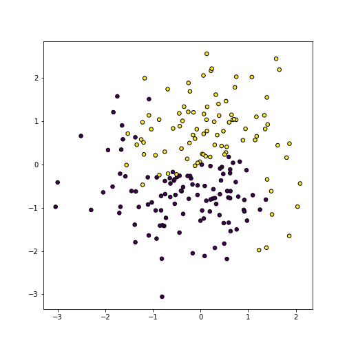
plot of chunk unnamed-chunk-61
Yin-Yang data.
First load it, and make a simple plot:
The plot shows data points of two different type (column c in the dataset), depicted by purple and gold colors. They are separated by a little fuzzy Yin-Yang style boundary.
Below, we will display how well do models capture the boundary.
12.4.2 How to display the decision boundary
In order to display the boundary, we’ll do the following:
- Fit a model that describes the color \(c\) as a function of \(x\) and \(y\). As decision boundary is mainly a predictive modeling tool, we’ll use sklearn for a large choice of predictive modeling tools.
- Create a large grid (e.g. \(100\times 100\)) and predict the color at each gridpoint. In order to do the prediction, we need to “straighten” (ravel) the rectangular grid into a data frame that contains only two columns (x and y).
- Make an image of the predicted colors. In order to make the image, we need to convert the vector of individual predictions back to a \(100\times100\) matrix.
- For better understanding, we may add the original data points to the image.
Here we’ll demonstrate the boundary with just logistic regression, but later we’ll use a similar plot to describe the behavior of other models too (see, e.g. Sections @ref(trees-classification-dboundary and 16.4). Now the tasks with the relevant code:
- Create the design matrix and fit the model
- Create the grid. More specifically, we need to create a data frame, containing columns x and y, that includes one line for every gridpoint. Here we use a \(100\times100\) grid:
x_min, x_max = X.x.min(), X.x.max()
# note: indexing assumes X is a data frame
y_min, y_max = X.y.min(), X.y.max()
## make a dense grid (nGrid x nGrid) in this extent
xx, yy = np.meshgrid(np.linspace(x_min, x_max, 100),
                     np.linspace(y_min, y_max, 100))
## Convert two grids into two columns
XX = np.column_stack((xx.ravel(), yy.ravel()))
XX = pd.DataFrame(XX, columns = ["x", "y"])
This gives us a new grid in the form of a data frame, each line of which corresponds to a gridpoint. Here is a small example:
##              x         y
## 7686  1.417632  1.256247
## 1263  0.225225 -2.375003
## 4624 -1.796683 -0.445901
## 208  -2.626184 -2.942386
Now we just use that data frame for prediction:
## array([0, 0, 0, 0])Now \(\hat y\) is the predicted color for each gridpoint.
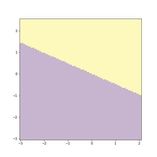
plot of chunk unnamed-chunk-65
- In order to display the predictions as an image, you need to
convert it back to a matrix. The dimension of the matrix should be
the same as for the grid we made above, so we can use one of its
components xx, and thereafter it can be displayed using
plt.imshow():
yhat = yhat.reshape(xx.shape)
_ = plt.imshow(yhat,
               extent=(x_min, x_max,
                       y_min, y_max),
               aspect="auto",
               interpolation='none',
               origin='lower',
               alpha=0.3)
There are multiple details you need to adjust with imshow(),
e.g. the coordinate values, aspect, and wheter the data starts from
lower or upper corner.
I prefer to plot the predictions in a pale color using alpha = 0.3,
e.g. 70% transparent palette. This makes it easier to see the data
points afterward.
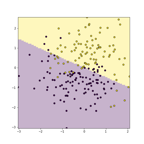
plot of chunk unnamed-chunk-66
Decision boundary that include both predictions (pale color background) and actual data points.
- Add data points to the figure. This can be done just with
plt.scatter(), but you probably want to ensure that it displays the same colors.
A few comments about the plot:
- You may want to plot only selected data points, only training data, or only validation data, depending on what do you want to show.
- This code is written assuming the data is submitted in the form of a
pandas’ data frame. If data is in the form of numpy arrays, then
you need to adjust certain contructs, e.g.
X.xshould be substituted byX[:,0]and so on.
12.4.3 Make a function to display the boundary
If you use decision boundary a lot, you may want to make a function for it. Here is a function that assumes data is provided as arrays, not as data frames. It has 4 arguments: a fitted model, design matrix X, outcome vector y, and number of grid points. This version assumes that X and y are numpy matrices, not pandas’ objects. The actual values are used for a) finding the extent of data to be plotted; and b) to be added to the actual plot, for visual guidance.
def DBPlot(m, X, y, nGrid = 100):
    ## find the extent of the features
    ## and add 'padding', here "1" to it.  Adjust as needed!
    x1_min, x1_max = X[:, 0].min(), X[:, 0].max()
            # note: indexing assumes X is a np.array!
    x2_min, x2_max = X[:, 1].min(), X[:, 1].max()
    ## make a dense grid (nGrid x nGrid) in this extent
    xx1, xx2 = np.meshgrid(np.linspace(x1_min, x1_max, nGrid),
                           np.linspace(x2_min, x2_max, nGrid))
    ## Convert two grids into two columns
    XX = np.column_stack((xx1.ravel(), xx2.ravel()))
    ## predict on the grid
    hatyy = m.predict(XX).reshape(xx1.shape)
    plt.figure(figsize=(8,8))
    ## show the predictions as an semi-transparent image
    _ = plt.imshow(hatyy, extent=(x1_min, x1_max, x2_min, x2_max),
                   aspect="auto",
                   interpolation='none', origin='lower',
                   alpha=0.3)
    ## add the actual data points on the image
    plt.scatter(X[:,0], X[:,1], c=y, s=30, edgecolors='k')
    plt.xlim(x1_min, x1_max)
    plt.ylim(x2_min, x2_max)
    plt.show()
We’ll use this or a similar function later in this book.
And here is an example how to use it:
This shows which areas are predicted as purple, and which ones as gold. The figure shows pretty clearly that the current tree splits the feature space into too detailed rectangles–it carves out single rectangles for individual purple and yellow dots. This is how it achieves the perfect accuracy, but as we only work on training data, it is obviously overfitting.
It may seem unnecessary to provide probabilities for both outcomes–after all, you can easily compute one from the other as they always sum to 1. But sklearn’s logistic regression can handle more than two categories (called multinomial logit), and in that case providing the probabilities for each individual outcome is quite useful.↩︎