Chapter 19 Neural Networks
This section discusses now to use neural networks in python. First we discuss multi-layer perceptrons in sklearn package, and thereafter we do more complex networks using keras.
We assume you have loaded the following packages:
We load more functions below as we introduce those.
19.1 Implementing a perceptron
In this section we implement perceptrons that perform logical AND and XOR. Both hare binary logical operations with the following results:
| x | y | x.AND.y | x.XOR.y |
|---|---|---|---|
| 0 | 0 | FALSE | FALSE |
| 0 | 1 | FALSE | TRUE |
| 1 | 0 | FALSE | TRUE |
| 1 | 1 | TRUE | FALSE |
19.2 Using scalars for coding perceptrons
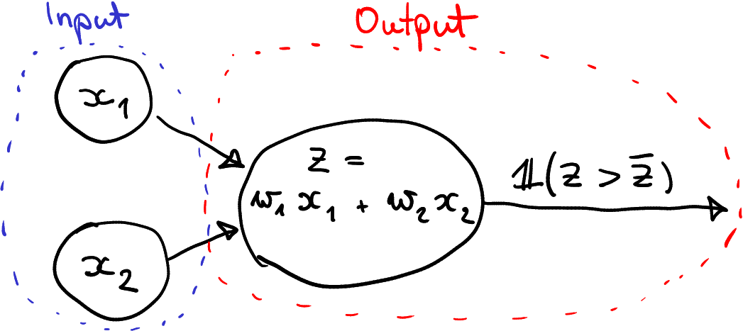
For a refresher, this is how a single node perceptron looks like. For logical AND operations, you can choose \(w_1 = 1\), \(w_2 = 1\) and \(\bar z = 1.5\).
This figure can be directly translated into the code:
x1, x2 = 0, 0  # pick the inputs (data)
w1, w2 = 1, 1
zbar = 1.5

## Compute
z = w1*x1 + w2*x2
y = (z > zbar) + 0  # convert to a number
y
## 0Exercise 19.1 In the example above, \(x_1\) and \(x_2\) were scalars. Will the code work if you replace these with vectors (numpy arrays) \(x_1 = (0, 0, 1, 1)\) and \(x_2 = (0, 1, 0, 1)\), as in the table above? Can you explain why?
19.3 Multi-Layer Perceptron
sklearn includes
multi-layer perceptrons, simple
dense feed-forward networks with an arbitrary number of hidden
layers. Even if simple in neural network context, they are still
powerful enough for many tasks. As with other models,
sklearn provides two functions: MLPClassifier for classification
tasks and MLPRegressor for regression tasks. This closely parallels
trees (see Section 16.1) and k-NN methods.
The basic usage of these perceptron models is similar to that of
all other sklearn models.
(See
Section 10.2.2 for introduction to sklearn
using linear-regression.)
The most important arguments for MLPClassifier are
Out of these, hidden_layer_sizes is the most central one. This describes
the network, in particular its hidden layers (the input and
output layers’ sizes are automatically
determined from data). It is a tuple that tells the
number of nodes for each hidden layer, so length of the tuple will
also tell the number of hidden layers. So for instance
hidden_layer_sizes = (32, 16) means two hidden layers, the first one
with 32 and the following one with 16 nodes.
activation describes the
activation function, choose “relu” (the default) unless you have good reasons to
choose something else. alpha is the L2 regularization parameter and
max_iter tells the maximum number of iterations (or epochs if
using SGD) before the optimization stops.
Below, we use color spiral data to demonstrate
MLPClassifier(). The task is, given the location, to predict the
color of the spiral arm.
First, load data and make the design matrix (out
of x and y, the location on plane), and outcome (the category
color):
spiral = pd.read_csv("../data/spiral.csv.bz2", sep = "\t")
X = spiral[["x", "y"]].values
y = spiral.color.values
Let’s start with a simple perceptron with a
single hidden layer of 20 nodes. Hence we use
hidden_layer_sizes=(20,), a tuple with just a single number.
Fitting the model and predicting is mostly similar to that of the other
sklearn so we do not discuss it here. We just
increase the number of iterations as the default 200 is too little in
this case:
from sklearn.neural_network import MLPClassifier
from sklearn.metrics import confusion_matrix

m = MLPClassifier(hidden_layer_sizes = (20,), max_iter=10000)
_t = m.fit(X, y)
yhat = m.predict(X)
confusion_matrix(y, yhat)
## array([[38, 52, 37, 1],
## [43, 50, 37, 4],
## [28, 45, 54, 2],
## [21, 41, 40, 7]])This simple model did not do well even on training data. Its accuracy is
## np.float64(0.298)This is because the model is too small for this complex pattern, just a single small hidden layer is not enough to model the complex spiral pattern well. Let’s also check to decision boundary plot (see Section 12.4.3) to see how does the model represent the image:
def DBPlot(m, X, y, nGrid = 100):
    x1_min, x1_max = X[:, 0].min() - 1, X[:, 0].max() + 1
    x2_min, x2_max = X[:, 1].min() - 1, X[:, 1].max() + 1
    xx1, xx2 = np.meshgrid(np.linspace(x1_min, x1_max, nGrid),
                           np.linspace(x2_min, x2_max, nGrid))
    XX = np.column_stack((xx1.ravel(), xx2.ravel()))
    hatyy = m.predict(XX).reshape(xx1.shape)
    plt.figure(figsize=(8,8))
    _t = plt.imshow(hatyy, extent=(x1_min, x1_max, x2_min, x2_max),
                   aspect="auto",
                   interpolation='none', origin='lower',
                   alpha=0.3)
    plt.scatter(X[:,0], X[:,1], c=y, s=30, edgecolors='k')
    plt.xlim(x1_min, x1_max)
    plt.ylim(x2_min, x2_max)
    plt.show()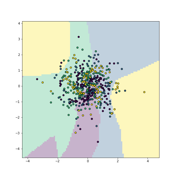
plot of chunk mlp-simple
Multilayer perceptron captures the main traits of the pattern.
We can see that the model correctly captures the idea: the data contains areas of different colors, but the shape of the areas is not accurate.
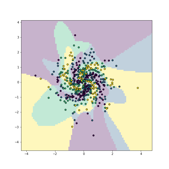
plot of chunk unnamed-chunk-10
Let us repeat the model with a more powerful network:
m = MLPClassifier(
    hidden_layer_sizes = (256, 128, 64),
    max_iter=10000)
_t = m.fit(X, y)
yhat = m.predict(X)
confusion_matrix(y, yhat)
## array([[103, 24, 1, 0],
## [ 26, 85, 22, 1],
## [ 0, 11, 86, 32],
## [ 0, 1, 11, 97]])## np.float64(0.742)Now the results are much better with the accuracy around 0.78 (on training data!). A visual inspection confirms that the more powerful neural network is quite good in capturing the spiral pattern in data.
Fitted network models have a number of methods and attributes,
e.g. coefs_ gives the model weights (as a list of weight matrices, one for
each layer), and intercepts_ gives the model biases (as a list
of bias vectors, one for each layer). For instance, the model fitted above
contains
## np.int64(452)biases. The second hidden layer’s weight matrix size is
## (256, 128)It has 256 rows because it has 256 inputs, and 128 columns because it has 128 nodes.
While sklearn offers easy access to neural network models, those models are substantially limited. For more powerful networks one has to use other libraries, such as keras, tensorflow or pytorch.
19.4 Keras and Tensorflow
Keras is a library (API) that is designed for building neural networks. It is a front-end library: it does not perform computations itself but relies on either tensorflow or pytorch backend to actually compute. However, it is much simpler to use the keras’ functionality, compared to building the networks from ground up. Keras allows the computations to be carried on GPU, potentially offering a big speed imprevements over CPU computations.
Keras’ functionality includes a wide variety of network layers where one can adjust the corresponding parameters. When constructing the network, one can just add the layers next to each other, connection between the layers will be taken care for by keras itself. A good source for keras documentation is its API reference docs.
Tensorflow can be hard and frustrating to install. Normally it
works fine using either conda install tensorflow or pip install tensorflow. However, sometimes things may go wrong and it may be
hard to find and fix the issues. In particular, pip normally installs
the most recent version, even if it is incompatible with the rest of
your packages. It also installs dependencies, and may upgrade
certain packages, breaking the python installation in the process.
In order to avoid messing with the
rest of your system, we strongly recommend to install it in a
virtual environment.
19.4.1 Example network in keras
Let us re-implement the color spiral example from the Multi-Layer Perceptron section but this time using keras. There will be a few differences we’ll discuss below:
- Construction of the network itself is different in keras.
- Keras does not compute the size of input and output layers from data. Both must be specified by the user.
- Finally, keras only predicts probabilities for all the categories, so we have to add code that finds the column (category) with maximum probability.
The full code can be downloaded from the Bitbucket repo, below we discuss the selected details only.
19.4.1.1 Building the Model
First, the most important step: building and compiling the model. This is very different from how it is done in sklearn. Let’s build a sequential model with dense layers, the same perceptron that we created using sklearn above in Section 19.3:
from keras.models import Sequential
from keras.layers import Dense, Input

# sequential (not recursive) model (one input, one output)
model = Sequential([
    Input(shape = (2,)),
    Dense(512, activation="relu",
          input_shape=(2,)),
    Dense(256, activation="relu"),
    Dense(64, activation="relu"),
    Dense(nCategories, activation="softmax")
])
We start with importing the functionality we need,
the model type (Sequential) and
two kinds of layers (Dense and Input).
Thereafter we create a sequential model in a somewhat similar fashion
as in sklearn by providing the layer descriptors to the
function Sequential().
Unlike in sklearn, the first layer should be the input layer.
This tells keras what kind of inputs to expect. Currently it
is just a tuple (2,) as our X-matrix only contains 2 columns. So
(2,) is just the shape of a single row of X, a single instance of
the input data. You can find the correct shape with X[0].shape.
But the input here does not have to be just a vector. For instance,
in case of images it may be a 3-D tensor with shape
(width, height, #color channels). You do not have to worry about
the inputs for the following layers, keras can figure it out itself.
Next, we include 3 dense layers. The first layer contains 512 nodes, the second one 256 and the last node contains 64 nodes. All these layers are fully connected (dense) and activated using relu function. If you forget to specify the activation function, keras by default will not use any activation and your complex model will be equivalent to logistic regression.
We also have to add an explicit output layer. As the task here is classification, we need as many output nodes as we have categories–we can compute this number as
Each output node will predict the probability that the input falls into the corresponding category. We can use softmax (multinomial logit) activation to ensure that the outcomes are valid probabilities. Note that in case of just two categories, softmax activation is equivalent to ordinary logistic regression. But unlike the ordinary logistic regression, we have a number of other layers preceding the last logistic layer.
Getting the input shapes and output nodes right is one of the major sources of frustration when starting to work with keras. The error messages are long and not particularly helpful, and it is hard to understand what went wrong. Here is a checklist to work through if something does not work:
- Do you include the input layer?
- Does the input shape correctly represent the shape of a single instance of the input data?
- Do you have correct number of nodes in the softmax-activated output layer?
See also Common Error Messages below.
19.4.1.2 Fitting the Model
The next task is to compile and fit the model. Keras models need to be compiled–what we set up so far is just a description of the model, not the actual model. The latter is code that uses tensors and can run on GPU if available. We can compile the model as
The three most important arguments are
lossdescribes the model loss function,sparse_categorical_crossentropy, essentially log-likelihood, is suitable for such categorization tasks where the different categories are coded as integers. Alternatively, if you use one-hot-encoded categories, you need to use just “categorical_crossentropy”.optimizeris the optimizer to use for stochastic gradient descent.adamandrmspropare good choices but there are other options.
The last line here prints the model summary, a handy overview of what we have done:
Model: "sequential"
┏━━━━━━━━━━━━━━━━━━━━━━━━━━━━━━━━━━━━━━┳━━━━━━━━━━━━━━━━━━━━━━━━━━━━━┳━━━━━━━━━━━━━━━━━┓
┃ Layer (type)                         ┃ Output Shape                ┃         Param # ┃
┡━━━━━━━━━━━━━━━━━━━━━━━━━━━━━━━━━━━━━━╇━━━━━━━━━━━━━━━━━━━━━━━━━━━━━╇━━━━━━━━━━━━━━━━━┩
│ dense (Dense)                        │ (None, 512)                 │           1,536 │
├──────────────────────────────────────┼─────────────────────────────┼─────────────────┤
│ dense_1 (Dense)                      │ (None, 256)                 │         131,328 │
├──────────────────────────────────────┼─────────────────────────────┼─────────────────┤
│ dense_2 (Dense)                      │ (None, 64)                  │          16,448 │
├──────────────────────────────────────┼─────────────────────────────┼─────────────────┤
│ dense_3 (Dense)                      │ (None, 5)                   │             325 │
└──────────────────────────────────────┴─────────────────────────────┴─────────────────┘
 Total params: 149,637 (584.52 KB)
 Trainable params: 149,637 (584.52 KB)
 Non-trainable params: 0 (0.00 B)
So this network contains almost 150,000 parameters, all of which are trainable.
After successful compilation we can fit the model:
In this example X is the design matrix, y is the outcome vector,
and the argument epochs tells
how many epochs to run the optimizer. Keras reports the progress
while optimizing, it may look like
Epoch 1/30
25/25 ━━━━━━━━━━━━━━━━━━━━ 2s 7ms/step - loss: 1.6020
Epoch 2/30
25/25 ━━━━━━━━━━━━━━━━━━━━ 0s 6ms/step - loss: 1.5531
Epoch 3/30
25/25 ━━━━━━━━━━━━━━━━━━━━ 0s 6ms/step - loss: 1.5257
Here you
can see the current epoch and the current
batch (for stochastic gradient descent).
We see the numbers 25/25 for batches because all epochs are run till
completion (25 batches). But when the estimation is ongoing, you
can see the batch number
progressing as the training proceeds. This
example works very fast, keras reports 2ms per step (batch) and
total time for epoch is too small to be meaningfully
reported. But a single
epoch may take many minutes for more complex models and larger
datasets.
Keras let’s you predict using model that is not fitted (unlike sklearn where that causes an error). The results will look mediocre at best.
19.4.1.3 Predicting and Plotting
When the fitting is done, we can use the model for prediction.
Prediction itself works in a similar fashion as in sklearn, just the
predict method predicts probability, not category (analogously to
sklearn’s predict_proba):
In this example, this will be a matrix of 5 columns where each column
represents probability that the data point belongs to
the corresponding category. Example lines of phat may look like
[[1.3339513e-37 5.6408087e-24 2.7101044e-10 1.2674906e-03 9.9873251e-01]
 [2.7687559e-09 1.9052830e-02 9.8094696e-01 2.3103729e-07 2.8597169e-19]
 [1.6330467e-18 6.0083215e-07 9.5986998e-01 4.0129449e-02 2.5692884e-08]
 [5.6379267e-15 1.8879733e-06 9.9859852e-01 1.3995816e-03 2.9565132e-11]
 [1.0658005e-19 7.9592645e-08 1.7678380e-01 7.8631145e-01 3.6904618e-02]]
In case of the first line, the largest probability, 0.998, is in the 5th column. In all three following lines, the 3rd column contains the largest probabilities, 0.981, 0.960, and 0.999 respectively, and finally, in the fourth line, the maximum value 0.786 is in the 4th column.
Usually we do not need the five probabilities but the actual
category–the column with the largest probability.
We can use
np.argmax(phat, axis=-1), it just finds
the location of the largest elements in the array, across the last
axis (axis=-1), i.e. columns. So for each row, we find the
corresponding column number. As typical for python, np.argmax()
counts columns starting
from 0, not from 1:
[4, 2, 2, 2, 3]Finally, we can compute confusion matrix in the same way as when using sklearn:
from sklearn.metrics import confusion_matrix

print("confusion matrix:\n", confusion_matrix(category, yhat))
print("Accuracy (on training data):", np.mean(category == yhat))
In this example we predict on training data but we can obviously
choose a different dataset. As the predicted value
will be a probability matrix of 5 columns, we compute yhat as the
column number that cointans the largest probability for each row.
The output may be look something like this:
confusion matrix:
 [[165  33   0   0   0]
 [  3  55  12   0   0]
 [  1  36 194   9   0]
 [  0   0  16  79   3]
 [  0   1   2  37 154]]
Accuracy (on training data): 0.80875
As you can see, the main diagonal dominates the confusion matrix, and accuracy is high.
Finally, if we want to make a similar decision boundary plot as
above (see Section 19.3),
then we
have to modify the DBPlot function in order to address
the different way to predict the category:
def DBPlot(m, X, y, nGrid = 100, fName=None):
    x1_min, x1_max = X[:, 0].min() - 1, X[:, 0].max() + 1
    x2_min, x2_max = X[:, 1].min() - 1, X[:, 1].max() + 1
    xx1, xx2 = np.meshgrid(np.linspace(x1_min, x1_max, nGrid),
                           np.linspace(x2_min, x2_max, nGrid))
    XX = np.column_stack((xx1.ravel(), xx2.ravel()))
    phat = m.predict(XX)  # 5 columns of probabilities
    hatyy = np.argmax(phat, axis=-1).reshape(xx1.shape)
    # one category for each gridpoint
    plt.figure(figsize=(10,10))
    _ = plt.imshow(hatyy, extent=(x1_min, x1_max, x2_min, x2_max),
                   aspect="auto",
                   interpolation='none', origin='lower',
                   alpha=0.3)
    plt.scatter(X[:,0], X[:,1], c=y, s=30, edgecolors='k')
    plt.xlim(x1_min, x1_max)
    plt.ylim(x2_min, x2_max)
    plt.show()
Again, the function is almost identical to the sklearn version,
except the line that computes hatyy
containing np.argmax(phat, axis=-1). This function converts
predicted probabilities to categories.
19.5 Image processing with convolutional networks
The main reason to choose keras over sklearn is its much more powerful toolset. This includes convolutional layers that are extremely helpful for image processing, and also tools to load data as you go, so one does not have to keep tens of thousands of images in memory.
We demonstrate the usage by categorizing images into cats and dogs.
The data used in this example can be downloaded from
kaggle. It contains
25,000 labeled training images and 12,500 unlabeled testing images (as
these are not labeled, those cannot be really used for testing). The
data sets are large (as is common for image processing), training data
is 600MB and testing data 300MB.
In
the code below we assume the images are located in cats-n-dogs/train
for training data. The full code example is on the Bitbucket
repo,
here we discuss just the more crucial parts of it.
19.5.1 Loading Data
Let us first set the model parameters:
imgDir = "cats-n-dogs"
imageWidth, imageHeight = 128, 128
imageSize = (imageWidth, imageHeight)
channels = 3
As we need to repeatedly find the images, we specify the location of
the folder here (you have to adjust this for your computer if you want
to run this program). Next, because the input tensors that correspond to
the images must be of the same size, we specify image target size here, and
resize all images later into shape imageSize (this will be done by
data generators, see below). In this example,
one color channel will be a \(128\times128\) matrix. We also specify that the images
contain 3 color channels, so a single image is in fact a
\(128\times128\times3\) tensor. Obviously, larger image size gives
better predictions but will be slower.
We do not want to load all images into memory–that would be a
very memory-hungry approach.9
Instead, we use the function image_dataset_from_directory(). This
function creates a keras dataset that is not loaded into memory, but
read from the disk batch-by-batch as needed:
from keras.utils import image_dataset_from_directory
## Dataset generators
trainDS, valDS = image_dataset_from_directory(
    imgDir + "train/",
    label_mode = "int",  # must match with 'sparse_categorical_crossentropy'
    color_mode = "rgb",  # color channels
    batch_size = 32,
    image_size = imgSize,
    shuffle = True,
    seed = 3,
    validation_split = 0.2,
subset = "both")- directory: the folder where the images are located. For correct labeling, the directory should contain subfolders, one for each category, that contain the images for that category. In this case, it should contain two folders, “cat” and “dog”, with the corresponding images inside.
- label_mode: “int” will give the numeric labels for the categories, here “cat” will be “0” and “dog” will be “1” as the categories are alphabetically ordered. If the label mode is “int”, model must be compiled with the “sparse_categorical_crossentropy” as its loss (see Section 19.5.3 below). If the label mode is “categorical”, the labels will be one-hot encoded with cat being \((1, 0)\) and dog \((0, 1)\), and it must be compiled with “categorical_crossentropy”.
- color_mode: can be “grayscale”, “rgb”, or “rgba”, the latter for png-images that include transparency.
- batch_size: how many images are read in one go. In this example, it reads 32 images, so the optimizer (stochastic gradient descent) will get \(32\times128\times128\times3\) input tensor for a single step.
- image_size: the desired image size. All images will be resized
to this size to ensure similar input tensors. Here we specify
(128, 128). - shuffle: whether to shuffle images when loading. It is useful to load the images in a random order when training, otherwise those are read in an alphabetic order. However, you do not want to shuffle validation data, otherwise the predicted and actual values do not match.
- validation_split, seed, subset: the data generator can
reserve part of the observations for validation. If this is the
case (
validation_splitis notNone), then you have to specify the random seed, and tell which subset (“training”, “validation” or “both”) you want to get. If both, it will return a tuple of training and validation subsets. In this example, we reserve 20% of images for validation, and return a tuple of both datasets (in the form of data generators).
While data generators are great for conserving memory, they are less well suited for certain other tasks, such as counting the number of cases or making a table of different categories. The following code prints how many cats and dogs are there in the training data:
yt = np.concatenate([y for x, y in trainDS], axis=0)
count = pd.Series(yt).value_counts().sort_index()
count.index = trainDS.class_names
print(count)
It uses a handy attribute of the data generator, class_names, to
convert the numeric categories (either “0”and “1”, or \((1, 0)\) and
\((0, 1)\)) into “cat” and “dog”.
Another handy attribute is file_paths, that one lists the file
paths (including folder names) of all the respective files. You can
easily count those, and use regular expressions to find their
category.
19.5.2 Building the Model
Now it is time to build the model. The basic model building steps are similar as discussed in Example network in keras: building the model, but this time we add more types of layers:
model = Sequential([
    Input(shape = (imgWidth, imgHeight, imgChannels)),

    Conv2D(32, 3, activation='relu'),
    BatchNormalization(),
    MaxPooling2D(pool_size=2),
    Dropout(0.25),

    Conv2D(64, 3, activation='relu'),
    BatchNormalization(),
    MaxPooling2D(pool_size=2),
    Dropout(0.25),

    Conv2D(128, 3, activation='relu'),
    BatchNormalization(),
    MaxPooling2D(pool_size=2),
    Dropout(0.25),

    Flatten(),
    Dense(256, activation='relu'),
    BatchNormalization(),
    Dropout(0.5),

    Dense(64, activation='relu'),
    BatchNormalization(),
    Dropout(0.5),

    Dense(2, activation='softmax')
])
We build a sequential model, but now the first three layers are convolutional layers. All layers, except the output layer, are activated using relu function.
The first layer is the input layer, describing how the inputs to the model look like. However, here we cannot use vectors—we cannot just flatten the image into an 1-D series of pixels because convolutions need information about the pixel locations. So we have to tell the model what is the image size and how many color channels are there. So here the input is not a data point on plane (a vector of length 2) but a \(128\times128\times3\) color image. So the input shape is a tensor of this shape.
The first convolutional layer (2-D convolutional layer) contains 32 filters of size \(3\times3\). This means we introduce 32 different convolutions and let the network learn which 32 filters give the best performance. As
stridesargument is not specified, these filters use \(1\times1\) strides, i.e. the kernel is moved over the images one pixel at time.This layer contains 896 parameters, \(3\times3\) kernel weights for each 32 filters and each 3 color channels, and 32 biases, one for each filter: \((3\times3\times3 + 1)\times 32 = 896\).
As the layer uses \(3\times3\) filters and no padding, it loses two image points at the edges. Hence the output is \(126\times126\times32\), the slightly shrunk image in 32 layers.
Convolutional layers are followed with the corresponding max pooling over \(2\times2\) image regions. As strides are not specified, they default to the same size as the pool, i.e. it uses \(2\times2\) strids. Finding maximum value does not need any extra parameters, but it halves the size of the input image because of strides two.
BatchNormalizationandDropoutare not separate layers but ways of training the corresponding layer’s weights. The former is useful to ensure stable gradients, the latter to avoid overfitting.The second and the third convolutional layer are similar to the first one, except that they contain more filters. These layers also contain way more parameters despite they are specified using \(3\times3\) kernel. Remember–the image itself contains three color channels, but the second convolutional layer works with the output of the first layer, i.e. 32 channels. Now the actual size of the kernel is \(3\times3\times32\) and hence we have \((3\times3\times32 + 1)\times 64 = 18,496\) parameters.
Final block of layers starts with image flattening. This means we transform 3-D tensors into an 1-D array of pixels. Spatial information is lost in the process. The flattened data is fed into the stack of two the dense layer with similar batch normalization and dropout.
Finally, we predict using two output nodes, activated through softmax function. This results in a \(1\times2\) vector of outcomes for each input image, the first one is the probability that the image depicts a cat, the second one that it depicts a dog.
19.5.3 Compile the model
The model must be compiled before it can be used. It is also useful to print its summary:
One can specify many parameters during the model compilation, e.g. the exact optimizer and its parameters, what statistic to print during the process, and so on.
The model summary will look like:
Model: "sequential"
_________________________________________________________________
 Layer (type)                Output Shape              Param #
=================================================================
 conv2d (Conv2D)             (None, 126, 126, 32)      896
 batch_normalization (Batch  (None, 126, 126, 32)      128
 Normalization)
 max_pooling2d (MaxPooling2  (None, 63, 63, 32)        0
 D)
 dropout (Dropout)           (None, 63, 63, 32)        0

 conv2d_1 (Conv2D)           (None, 61, 61, 64)        18496
 batch_normalization_1 (Bat  (None, 61, 61, 64)        256
 chNormalization)
 max_pooling2d_1 (MaxPoolin  (None, 30, 30, 64)        0
 g2D)
 dropout_1 (Dropout)         (None, 30, 30, 64)        0

 conv2d_2 (Conv2D)           (None, 28, 28, 128)       73856
 batch_normalization_2 (Bat  (None, 28, 28, 128)       512
 chNormalization)
 max_pooling2d_2 (MaxPoolin  (None, 14, 14, 128)       0
 g2D)
 dropout_2 (Dropout)         (None, 14, 14, 128)       0

 flatten (Flatten)           (None, 25088)             0
 dense (Dense)               (None, 256)               6422784
 batch_normalization_3 (Bat  (None, 256)               1024
 chNormalization)
 dropout_3 (Dropout)         (None, 256)               0

 dense_1 (Dense)             (None, 64)                16448
 batch_normalization_4 (Bat  (None, 64)                256
 chNormalization)
 dropout_4 (Dropout)         (None, 64)                0

 dense_2 (Dense)             (None, 2)                 130
=================================================================
Total params: 6534786 (24.93 MB)
Trainable params: 6533698 (24.92 MB)
Non-trainable params: 1088 (4.25 KB)
_________________________________________________________________
It is instructive to analyze and understand the number of parameters and the output shapes. We can see that the model contains over 6.5M parameters, most of which are in the first dense layer. This is because all the output pixels of the third pooling layer (\(14\times14\times128\)) must be fed into all 256 nodes of the dense layer. Hence we have \(256 \times 14 \times 14 \times 128 = 6,422,528\) weights and 256 biases, this is exactly 6,422,784 parameters for the dense layer.
We can also see how image size is decreasing through the convolutional
layers. Remember, the input images are \(128\times128\) pixels. As the
convolutional filters are \(3\times3\) pixels large, each of them cuts
two pixels off from the image (as we did not specify any padding),
and hence the first conv2d layer
outputs \(126\times126\) pixels. Max pooling over \(2\times2\) squares
further halves the image size to \(63\times63\). If we had specified
strides larger than one, we would reduce the size even more rapidly.
19.5.4 Train the model
Training the model works in a similar way as for the example network above (see Section 19.4.1.2). The only exception is that instead of the design matrix, the data is fed in the form of a keras dataset. As we explained above, the dataset is not in memory, but loaded from disk as needed (see Section 19.5.1).
As complex models, such as distinguishing cats and dogs, are much slower to fit, the example code only uses a single epochs. But for better results, you may need to train it for dozens of epochs.
19.5.5 Common model errors
Keras’ errors may be hard to understand for the un-initiated. Here we describe a few common errors. Note that these may be buried inside of large list of messages, usually toward the end.
19.5.5.1 Wrong input shape
Beginners often do not understand the input shape. But it is a necessary part of information that must be fed to the model. If we get it wrong, for instance if we specify the first layer as
model.add(Conv2D(32,
                 kernel_size=3,
                 activation='relu',
                 input_shape=(imageWidth, imageHeight)))  # no channels!
Then keras responds with a message
ValueError: Input 0 of layer conv2d is incompatible with the layer:
expected min_ndim=4, found ndim=3.
Full shape received: [None, 128, 128]
This tells that a Conv2D layer expects a 4-D tensor as its input (min_ndim=4). The correct shape should be [None, 128, 128, 3], where None means that the different cases (different images) that are stacked along that dimension.
This error happens during the model building, i.e. when you call
model.add(Conv2D(...)).
Sometimes you get the number of input extents right, but their dimension wrong. For for instance, if you specify 5 color channels instead of 3:
model.add(Conv2D(32,
                 kernel_size=3,
                 activation='relu',
                 input_shape=(imageWidth, imageHeight, 5)))  # should be 3 channels!
then the error will be
tensorflow.python.framework.errors_impl.InvalidArgumentError:
input depth must be evenly divisible by filter depth: 3 vs 5
It tries to wrap the \(128\times128\times3\) image into the \(128\times128\times5\) tensor, but it does not fit well.
This error occurs first when the fitting algorithm discovers that the
images contain 3 channels instead of 5, i.e. when you call
model.fit.
19.5.5.2 Wrong number of categories
This problem is conceptually fairly easy to grasp: the number of nodes in the final softmax layer must equal to the number of categories. If we get this wrong, e.g. by specifying the last layer as
then keras produces
tensorflow.python.framework.errors_impl.InvalidArgumentError:
logits and labels must be broadcastable:
logits_size=[32,3] labels_size=[32,2]
This tells that we were requesting 3 nodes (3 “logits”), but the data (labels) only contain 2 different categories. “32” is batch size here, that is why it replies not “3” and “2” but as “[32,3]” and “[32,2]”.
This error occurs when the fitting algorithm finds that there are too
few categories, i.e. when you call model.fit.
19.5.5.3 Image runs out of pixels
Each convolutional filter makes the image smaller because we lose pixels at the edges (unless we use padding). If we use strides that are larger than one, we also lose output pixels because we now move with larger steps. In a similar way, pixels get lost in pooling because pooling layers “pool” pixels over neighboring areas into a single one. In this way it may happen that the image does not contain any pixels at a certain stage.
Let’s demonstrate it by adding strides=3 to all convolutional layers. The first layer now looks like:
model.add(Conv2D(32,
                 kernel_size=3,
                 strides=3,
                 activation='relu',
                 input_shape=(imageWidth, imageHeight, channels)))
The image gets too small–after a few operations it contains no pixels. keras stops with
ValueError: Negative dimension size caused by subtracting 2 from 1
for '{{node max_pooling2d_2/MaxPool}} = MaxPool[T=DT_FLOAT,
data_format="NHWC", ksize=[1, 2, 2, 1], padding="VALID",
strides=[1, 2, 2, 1]](batch_normalization_2/cond/Identity)'
with input shapes: [?,1,1,128].
If you notice such a “negative dimension size” error, then you should check your “Output Shapes” in the model summary (see Section 19.5.2 above). Remove all convolutional layers besides the first one and try to understand what will be the image size after each operation, and which operations you want to remove or modify to retain an image with a meaningful number of pixels.
This error occurs at the model compilation stage where keras is computing size of the tensors.
19.5.6 Training the model
Now is time to setup training data generator that reads files during the model fitting:
## Training data generator:
train_generator = ImageDataGenerator(
    rescale=1./255,
    rotation_range=15,
    shear_range=0.1,
    zoom_range=0.2,
    horizontal_flip=True,
    width_shift_range=0.1,
    height_shift_range=0.1
).flow_from_dataframe(
    df,
    os.path.join(imgDir, "train"),
    x_col='filename', y_col='category',
    class_mode='categorical',  # target is 2-D array of one-hot encoded labels
    target_size=imageSize,
    shuffle=True
)
ImageDataGenerator is a class that can handle images in
various ways, in particular it can rescale the intensity from 0-255
integer range to 0-1 float range, and it can introduce various small
modifications to the image, such as rotation and shear. This is
useful for adding more variation to the training data. However, do
not modify your test data! We also shuffle the training data in order
to avoid feeding it always in the same order to the network.
After introducing modifications to the image, we call method
flow_from_dataframe. It takes
the data frame that contains both images (specified as x_col) and
labels
(specified as y_col) and tells how the data should be read. In this case we
request
the images to be converted to the target
size. class_mode tells keras to convert category into one-hot
encoded matrix, the shape needed by the model.
It is possible to add another similar data generator for validation data, so keras will output current information not just about training accuracy but also about validation accuracy when the model is running. However, we do not do it here for simplicity.
Now we can proceed with model training:
model.fit method is somewhat similar to that of sklearn, but it
accepts a lot more options. Here we provide training data generator,
and tell how many epochs to train.
One epoch is usually too little, but more epochs may be slow. In case
of this network and data, a single epoch will give you accuracy of
approximately 60% while 40 epochs will reach to 95%.
Model fitting returns a history object which contains information
about training loss and accuracy, and if validation_data is provided
(as it is here), then it also shows validation loss and accuracy.
19.5.7 Predictions and Validation
The following step is to predict the category on testing data. We proceed in a similar way, by creating a data generator that reads files as specified in the data frame:
testDir = os.path.join(imgDir, "test")
dfTest = pd.DataFrame({
    'filename': os.listdir(testDir)
})
print(dfTest.shape, "test files read from", testDir)

test_generator = ImageDataGenerator(
    rescale=1./255
    # do not randomize testing!
).flow_from_dataframe(
    dfTest,
    os.path.join(imgDir, "test"),
    x_col='filename',
    class_mode = None,  # we don't want target for prediction
    target_size = imageSize,
    shuffle = False
    # do _not_ randomize the order!
    # this would clash with the file name order!
)
In an analogous fashion as when we created training data, we first
list the image files in the folder, and create the corresponding data
frame. However, as these images are not labeled, we do not have
“category” variable here, this is also why we specify
class_mode=None.
We do not want testing images distorted or
shuffled either. Shuffling the test images will break the
correspondence between labels and images, and give essentially random
accuracy.
We can predict the probabilities just be feeding the test generator to
model.predict:
phat = model.predict(test_generator)

dfTest['category'] = np.argmax(phat, axis=-1)
label_map = {0:"cat", 1:"dog"}
dfTest['category'] = dfTest['category'].replace(label_map)
phat will be the predicted probability matrix, with the first column
describing the probability that the image is a cat, and the second
column is the probability that the image is a dog. It may look like
[[0.5337883  0.46621174]
 [0.4693922  0.53060776]
 [0.10248788 0.89751214]
 [0.05728473 0.9427153 ]
 [0.6855554  0.31444466]]
In this example the first image is more likely a cat (\(p = 0.53\)), but the algorithm is not really sure. However, the fourth example is confidently a dog (\(p = 0.94\)). The last three lines find the category of maximum probability, and replace the 0/1 labels with cat/dog labels for easier reading the results.
The final part of the code also plots a random set of images with the corresponding labels, after resizing those to the same desired image format so you see what kind of images the computer was working with!
19.5.8 Analyzing the model
You can get the layer data out of fitted models with
This returns a large number of parameters for the layer called conv1.10 One of these is weights, a list with two components: filter weights (the first component) and filter biases (the second component). We can extract the weights as
This returns an array of \(S_x \times S_y \times N_L \times N\) where \(S_x\) and \(S_y\) are the x- and y-size of the filter, \(N_L\) is the number of layers for the filters, and \(N\) is the number of filters. For instance, if the first convolutional layer contains 50 filters of \(4\times4\) size, and the input is 3-layer color image, then the corresponding weights is an \(4\times 4\times 3\times 50\) array.
19.6 pytorch
In recent years, pytorch has become more popular than keras. This section gives the basic introduction to that library.
pytorch is internally called torch, so you need to import torch,
not pytorch. This is also true for installation, it can be done
with pip install torch, not pytorch.
Pytorch allows to build neural networks from scratch, layer-by-layer. It also includes a plethora of more advanced tools, such as transformer layers and gpu acceleration. However, such power-user tools may feel overwhelming for beginners.
Torch requires that all data are converted to torch tensors, and maybe back to numpy if you want to use the results later with the basic python. Without additional actions, these tensors live in the main memory and computations are done by CPU. However, if you have a GPU, you can transfer the tensors over to the gpu and run the models by GPU. This may offer a substantial speed boost for certain tasks. By default, only NVIDIA CUDA framework is supported but modern AMD Radeon cards work very well too using its ROCm framework (the support needs to be installed separately though).
19.6.1 Color spiral using torch
This section discusses how to build a simple multi-layer perceptron using pytorch and the same spiral data as Section 19.3. It only provides the most important parts of the code, the full code is available in Bitbucket.
19.6.1.1 Setting up data
To begin with, you need to create your design matrix X and the outcome vector y. I also count the number of categories as that number is needed to build the last layer:
Note how the outcomes are built as spiral.color.values - 1. This is
because the dataset contains categories 1-4, but torch assumes the
values start from 0, and hence you need to convert those to 0-3.
Next, you need to load the modules:
This imports the basic torch functionality, its neural-network related module, and the optimizers.
As the final step of the setup, you need to convert numpy matrices to torch tensors:
X_tensor = torch.FloatTensor(X)  # 32-bit float data type
y_tensor = torch.LongTensor(y)  # 32-bit int data type
Now your data are ready to be entered into a torch model.
19.6.1.2 Building the model
The three hidden-layer model can be built by just adding layers to
nn.Sequential():
input_size = X.shape[1]  # 2 currently, x and y
model = nn.Sequential(
    nn.Linear(input_size, 512),  # 2 inputs to input layer, 512 nodes
    nn.ReLU(),  # ReLU activation
    nn.Linear(512, 256),  # 512 previous nodes give input to this layer
    nn.ReLU(),
    nn.Linear(256, 64),
    nn.ReLU(),
    nn.Linear(64, nCategories)
    # nn.Softmax()
)
Construction of the model is fairly intuitive:
The model can be constructed using
Sequential()but just passing various layers to it in the correct order. Note that its argument is a list of layers, not code: there must be commas between the functions.Sequential()connects the layers as needed, i.e. it feeds output from the previous layer as input of the following layer.In order to build the first layer (
nn.Linear(input_size, 512)) we need to know the dimension of the input. Here it is just “2”, i.e. we feed a vector of length 2 to the first layer. Or rather–it will be a matrix of 2 columns a number of datapoints.Linear()is a layer that just computes the linear transformation (essentially a linear regression).In a similar fashion, the activation functions
ReLU()andSoftmax()just apply the corresponding non-linear transformations to the inputs.However, because
CrossEntropyLoss()automatically includes softmax transformation (see below), I have commented this line out.
Finally, we also need to specify the loss function and the optimizer:
Cross-entropy loss (log-likelihood) is a good approach for classification problems, and Adam is a modern stochastic gradient descent-based optimizer.
19.6.1.3 Training the model
Training is maybe the most complex task when using torch. There are several concepts you should know.
- The model can be in training mode and evaluation mode (default).
For evaluation, you want it to be in evaluation mode. This is
because certain layers, such as dropout and batch normalization,
work differently while training (they are active) or evaluation
(they are not involved). One can switch between modes with
model.train()andmodel.eval(). - torch automatically computes gradients. However, each time you
compute a gradient, it does not return the new gradient but it
accumulates gradient values–hence what you get is old gradient plus
new gradient. Because this is not what you usually want, you have
to zero the gradients before compute the new ones, either using
optimizer.zero_grad()ormodel.zero_grad().
You need to explicitly run the training loop, in this example 100 times (this gives training accuracy 0.6..0.7):
for epoch in range(100):
    ## Forward pass
    outputs = model(X_tensor)
    loss = criterion(outputs, y_tensor)

    ## Backward pass
    model.train()  # switch to training mode
    optimizer.zero_grad()
    loss.backward()
    optimizer.step()

    model.eval()  # switch to evaluation mode
The loop does a number of tasks:
- It computes predictions
outputsgiven inputsX_tensor, and based on the predictions and the criterion, it computes the loss. (In terms of data structure, both of these are torch tensors.) - The model is switched to training mode for gradient-based parameter
updates
(backpropagation):
model.train(). - Former gradients are deleted:
optimizer.zero_grad(). - The gradients are calculated:
loss.backward(). The gradients are calculated automatically through the compute graph that is part of torch tensors. - The weights are updated:
optimizer.step(). The gradient descent methods only need the gradient and the current weight values in order to update the weights. Some optimizers may do a fair amount of book-keeping in the process, e.g. to compute optimal learning ratio and to approximate the Hessian matrix. - Finally, the model is switched back to evaluation mode:
model.eval().
19.6.1.4 Calculating the accuracy
Computing accuracy involves predicting the values. model(X_tensor)
runs the model on all X values and returns a matrix of
probabilities. Thereafter we use torch.max(..., 1) to find the
maximum category. Finally, accuracy is calculated from that category.
with torch.inference_mode():
    yhat = model(X_tensor)
    _, yhat = torch.max(yhat, 1)
A = np.mean(yhat.numpy() == y)- First, we use
torch.inference_mode()for inference. This makes torch not to calculate the gradients, and hence the inference will be faster and less memory hungry. model(X_tensor)computes probabilities for all categories and returns a \(N\times C\) matrix where each rows is a data point and each column is the probability of the corresponding category.- As we are not interested in probabilities but the predicted
category–the category that has the largest probability, we use
torch.max(..., dim = 1). This returns a tuple of probability values and the corresponding categories.dim = 1tells that we are not interested in the overall maximum but the maximum category for each row. This will be stored to yhat. - Finally, accuracy is computed using numpy tools after converting yhat to a numpy array. As this is just numpy, these calculations are taken out of the inferece_mode block.
19.6.1.5 Decision boundary plot
With torch, the basics of the decision boundary plot is the same as when using sklearn (see Section 12.4.3). The only difference is in how you predict the values on the grid, and how you compute the predicted category.
Here are the lines that differ from the sklearn’s version:
def DBPlot(model, X, y, nGrid = 100):
    ## ...
    XX = np.column_stack((xx1.ravel(), xx2.ravel()))
    model.eval()
    with torch.inference_mode():
        phat = model(torch.FloatTensor(XX))
        _, hatyy = torch.max(phat, 1)
    hatyy = hatyy.numpy().reshape(xx1.shape)
## ...- First, in order to predict on the grid XX, the model is switched
to the evaluation mode
model.eval(). - Second, the inference is done in inference mode where the gradients
are not calculated
with torch.inference_mode() - the most important command is
phat = model(torch.FloatTensor(XX)). This computes the predictions on the grid XX (after converting it to a tensor). - thereafter,
torch.max(phat, 1)returns the maximum probability categories for each gridpoint (as a torch tensor). - Finally, the categories are converted to numpy as reshaped to the original grid form.
The rest of the code is exactly the same as in case of sklearn.
One \(128\times 128\times 3\) image contains 16,384 pixels. With three color layers, it amounts to 49,152 color values. If stored 8-bits per pixel (common in for jpeg images), all 25,000 images amount to approximately 1.2GB.↩︎
You can see layer names with
model.summary(). See Section 19.4.1.2. You can also give each layer a name of your choice with the argumentname, e.g.Conv2D(..., name = "conv1").↩︎