Chapter 2 Python
TBD: remove section number from “intro”
Python is a general programming language which in recent years has gained a lot of popularity. It is in many ways similar to C++ and java, but avoids a number of complexities of those languages. However, it also includes a number of power-user tools, such as passing by reference, that allows it to handle data more efficiently than more functional languages like R. Unlike C++ or java (and like R), python is weakly typed and skips much of the other rigor of those language, so it is a much better choice for quick scripting and prototyping.
Python has a rich infrastructure of libraries, including data science-related libraries. Although powerful, not all of those are simple to learn. Part of the problem is not related to python or the libraries per se, but to the fact the data-processing concepts are complex. The other source of the complexity are the power-user tools that are designed for power-users, not for beginners. For instance, many python libraries have options to modify data “in place”, i.e. without doing a copy in memory. This is sometimes very handy, in particular when handling large data structures. But it is also a source of frequent confusion. The third source of problems is related to rapid development of certain popular frameworks. For example, tensorflow is developing rapidly with an unfortunate result of breaking the old code. If you haven’t been continuously updating your code for last few years, expect to run into problems now.
Finally, due to the rapid development, python itself is also rapidly changing. This may easily lead to installation hell, where the user has to keep different versions of python installed in order to support old versions of libraries as some of the code only works with older versions. There are tools, such as anaconda environments or python virtual environments that make this process simpler, but unfortunately all too often it happens that the different versions still manage to disturb each other somehow.
2.1 Installing python
As python is a popular tool for operating system (OS) related tasks, many OS-s may already have a version of python installed. Check your computer package manager.
However, for consistency in data science it is often preferred to install anaconda. Anaconda is a consistent set of packages that contain python, popular data science libraries, and many other related tools. You need to download anaconda installer and run in on your computer. Choose the default options unless you know what you are doing.

Anaconda navigator in Windows 10 environment.
On windows and mac OS-s, anaconda install anaconda navigator, a graphical interface that let you access the most important anaconda related programs. This includes jupyterlab and jupyter notebooks for interactive coding, spyder text editor that is somewhat similar to RStudio, just for python, and anaconda-aware command line interface. The latter is useful if you want to run python program from command line.
Anaconda also allows to keep different versions of python and other packages installed at the same time through environments, you can imagine environments being different folders that contain different versions of the software. However, if it is the first time you install anaconda on your computer then you don’t have to set up environments.
2.2 How to Use Python
2.2.1 Command line
~/d$ python hello.py
 Hello!
  Hello!
   Hello!
    Hello!
     Hello!
:-)
~/d$
~/d$ cat hello.py
#!/usr/bin/env python3

for i in range(5):
    print(" "*i, "Hello!")
print(":-)")
~/d$
Running python code from command line. The program,
printed below with cat command prints five times the word “Hello!”.
Python can be used in different ways. The traditional way is to use a text editor or IDE to write a python program (typically using .py as the file extension), and running the program from command line. Modern IDE-s also support code execution with a single click. Command line is the preferred way to run python code (or any other program code for that matter) for tasks that take long time or run as backend without user interaction. If you use anaconda, you should use the respective anaconda command prompt to run python programs.
2.2.2 IPython: interactive python
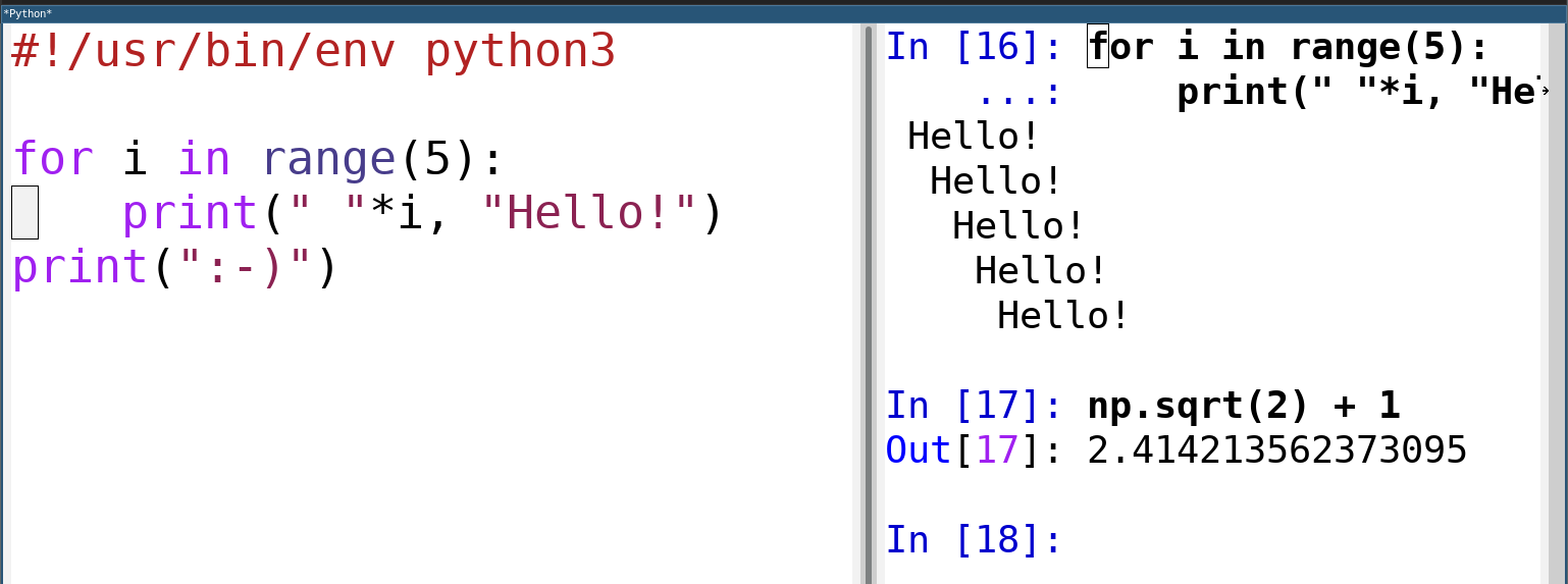
The same program as above in an emacs window, next to the ipython console that shows its output. One can use ipython console for various quick calculations, and for running programs chunk-by-chunk (note that the last print statement has not been executed). Many programming editors support ipython.
Alternatively, python has powerful and rich support for console
operations through ipython, the interactive python. It supports a
number of macros, such as %timeit for timing command evaluations,
and other goodies designed for interactive evaluation. Ipython is
normally used in combination with a text editor, such as spyder that
allows to write code and execute it easily through ipython. Spyder
is included in anaconda installation and reminds in many ways RStudio.
2.2.3 Jupyter notebooks
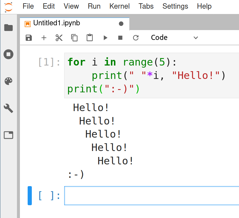
The same program as above running in a Jupyter notebook (through Jupyterlab). The code is in the code cell, output of it is visible underneath.
In recent years, it has become increasingly popular to use python through an interactive web-based environment jupyter notebook. Notebooks consists of code cells and markdown cells. Code cells can contain code which can be executed with a simple click (or keyboard shortcuts, e.g. Shift-Enter). The code is executed through ipython, so ipython tools are available in notebooks too. The markdown cells contain markdown text and can be rendered by a similar click or shortcut. The big advantage of notebooks is the immediate feedback, one can write the code a few lines at time, execute these, and immediately correct for potential errors. But notebooks are not a solution for every problem. In particular, one may prefer to run complex tasks without user interaction. Notebooks also permit to run cells out-of-order and in this way they can cause errors you do not see in traditional coding.
Notebooks are the most popular way for literate programming in python. One can easily mix code, output, and textual explanations in notebooks, and convert the result into html pages or a pdf document.

Jupyterlab icon
In order to use notebooks, one has to start the notebook server, typically by clicking on the Jupyterlab icon on the Anaconda navigator window. This opens a new browser window where one can start a fresh notebook (or open an existing one). Notebooks can also be set up to run on a server instead of local computer, in that case one has just to point the browser to the dedicated start page.
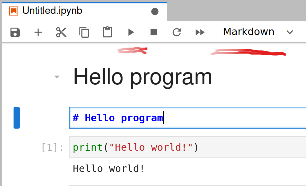
Adding markdown to notebooks. One can choose cell type from the drop-down menu at top-right, and afterward render the markdown with the arrow icon (both underlined), or more likely with Shift-Enter.
The notebook cells can contain either code or markdown text. The figure at right show three cells in Jupyterlab. The middle cell, marked with a blue bar at left, is the active cell where one can write and edit text. This is currently a markdown cell, as visible on the top-right dropdown menu (underlined in red). When you execute the markdown using the “run” triangle (top center, underlined in red), or more likely by Shift-Enter, the markdown will be rendered. A similar, rendered cell is visible as the topmost cell in the notebook.
Underneath, we can see a code cell that has already been run. Code cells can be recognized by the brackets at left, the number “1” within brackets means that this cell was run as the first cell in this notebook. If the code produces any output, this is also visible underneath. The visual layout and menus are somewhat different when using notebooks outside of Jupyterlab.
Jupyter notebooks share a number of similarities with rmarkdown but there are also a number of differences. Both are frameworks for literal programming and both support different programming languages, including python and R. However, notebook file format contains output while rmarkdown does not contain it. This makes notebooks an easy way to share both code and output. But output in the file makes it less suitable for version control systems, and the file format is also much more complex. The table below summarizes the main differences between these two formats.
| Jupyter notebooks | rmarkdown |
|---|---|
| Separate code cells and markdown cells | code chunks in markdown text |
| Includes output | does not include output |
| Json file containing text, code, output | markdown file containing text, code (no output) |
| Not git friendly (because of output) | git friendly |
| Works in browser | works in RStudio |
| Limited support elsewhere | can be used with different text editor (just text) |
| Requires background process running (kernel) | requires compilation (or RStudio) |
As a practical implication, with notebooks you can inject html into your output and in this way create virtually unlimited webpages. However, a few simple tasks, such as writing text, is just a bit more complicated (new cells are code cells by default), so notebooks discourage writing. Notebooks also do not include easy inline code chunks that are possible with rmarkdown.
2.3 Base language
The base python is well designed and easy to learn. It is in many ways similar to C++ and java, but much simpler. It also lacks some of the rigor of the those languages which makes it a very good choice for scripting and quick prototyping but a somewhat less suited for complex large-scale projects.
2.3.1 A few words about variable names and coding style
Before getting into the specifics of python, a few general remarks about coding style. There is always a myriad of ways to choose variable names, naming schemes, and algorithms. This is often of little importance but may sometimes lead to errors that are frustratingly hard to debug. Below we discuss a few general strategies. As always, feel free to break any of these rules, but be able to explain why do you do that!
2.3.1.1 Choose appropriate variable names
What is “appropriate” depends on the task. If you are writing a
tiny loop that prints a message three times, the loop counter can well
be called i:
The plain i makes the code easier to grasp than a more complex name,
e.g. greeting_counter. Just compare:
However, this does not mean that you should always choose the simplest
variable names. greeting_counter may be a good choice in case you
are developing a more complex project with nested loops and many counters,
and you need to know what exactly the loop is counting.
2.3.1.2 Do not overwrite data with derived results
Data science tasks typically start with loading, cleaning and filtering data along the lines
## load
data = pd.read_csv("data.csv")
# check if loading was successful
...
## clean
data = data.dropna(["var1", "var2"], axis=1)
# do more cleaning...
...
## subset
data = data[data.var3.isin(interesting_cases)]
# do more subsetting...
## start real work here
This is a good way to work if you are running the code from command
line in batch mode. However, in notebooks where typical workflow
jumps back and forth, it may lead to confusing issues where a piece of
code that just a second ago worked perfectly does not work any more,
or produces wrong results. In the example above, if you run the
cleaning code
again, you’ll get an error
telling you that variables var1 and var2 were not found.
Consider creating temporary variables (and
deleting those with del afterwards if needed).
2.3.1.3 Create a naming scheme for collections and elements
Another common task is to run a loop over all elements of a collection. The collections usually have a particular meaning and hence you tend to call it accordingly. But the individual elements you extracts in the loop have a rather similar meaning, and you are tempted to call it something very similar.
Consider a confusing example:
friend = ["Li Seming", "Gao Guoqin", "Wang Chengbi"]
for person in friend:
    ...
    ## what is person, what is friend?
    ## which one is collection, which one is element?
    ## are they related in the first place?
There are two problems with the chosen names: a) they are both in
singular, so it is unclear which one is an element and which one is
the collection; and b) they are quite different, so it is not clear if
person and friend are somehow related. An alternative would be to
consistently use the -s plural ending, or maybe _list suffix:
friends = ["Li Seming", "Gao Guoqin", "Wang Chengbi"]
for friend in friends:
    ...
    ## friends: plural, hence collection
    ## friend: singular, hence element of 'friends'
Select a coherent naming schema that distinguishes collections from their elements!
2.3.1.4 If you change the variable meaning, change its name too
Consider a task: we have test score data between 0 and 100. We want to replace this with a simple variable, just a binary indicator that tells if someone received score over 80. Sometimes we see it coded as
Why is it confusing? Because the original “testscore” means numeric score between 0 and 100. But now further down in the code it suddenly means a logical value for high test score.
In such case create a new variable, such as “highscore”. If you are worried about memory footprint then you may remove the original variable.
2.3.1.5 Select appropriate names for complex concepts
Normally you pick variable names that closely resemble the corresponding concept names. Now consider you are doing Bayesian statistics, and you need to compute probabilities \(\Pr(S = 1)\), \(\Pr(S = 0)\), \(\Pr(W = 1|S = 1)\), \(\Pr(W = 0|S = 1)\), \(\Pr(W = 1|S=0)\) and \(\Pr(W = 0|S = 0)\). These are probabilities and conditional probabilities, written down in standard mathematical notation. How would you name these six related but still very distinct variables? As you can see, the notation is confusingly similar but the small differences are still very important. You must be able to tell from your variable names which concept does it describe. I’d suggest to use names that reflect the mathematical notation as much as possible, that are close enough that both you and whoever else may read your code understands which concepts they are referring to. For instance, you can choose
Pr_S1, Pr_S0, Pr_W1S1, Pr_W0S1, Pr_W1S0, Pr_W0S0Complex formulas may be confusing to begin with, and introducing
incoherent variable names only adds to this confusion. It is also
extremely hard to debug code where one has to guess and remember
that pw_second means \(\Pr(W=0|S=1)\) and probability_new2 is \(\Pr(W=0|S=0)\).
2.3.1.6 Use grammatically correct words
Computer does not care about your English grammar. But there is only
one way to write the words correctly while you can write them wrong in
a myriad of different ways. It is just hard to remember if middle
point should be written as middlePoint, mdlePoint, midPoint or
midlPoint… If someone else is reading your code, they
may not understand if this is a typo or correct variable name.
Typos in variable names is a frustrating source of errors that may take hours or even days to debug. In particular, long variable names in languages that do not require explicit declaration can contain typos that are surprisingly easy to overlook. Do not make this work harder by intentional misspelling!
2.3.2 Code blocks
One of the most distinct element of python language is the use of code blocks–instead of using braces or keywords, code blocks in python are defined by indentation. Consider the example:
The for-loop embraces three lines of code, marked by an extra indent (typically 4 spaces): the first print-statement, and the if-statement that in turn is made of two lines. The if-statement inside the loop contains the if-condition itself, and besides that just one additional line, marked by additional indent (4 more spaces). The last print-statement is indented by the same amount as the for-statement (i.e. not indented at all), and hence belongs to the same code level, here to the main program itself. It gives the following result:
## 0
## 1
## 2
## 3
## too much
## doneSimilar indentation rules apply to all code blocks, including function
definitions, and exception handling with try and except: the block
starts with a colon at the end of the declaration line (for and
if-lines in the example), and is defined by extra indentation.
2.3.3 Variables and assignment
The most important data types are floats (floating-point numbers), integers, logicals, and strings. The following example demonstrates all these data types:
a = 1.0  # double
b = 2  # integer
λ = False  # logicals are 'False' and 'True'
s = 'text'  # string, can also use double quotes
A float is created by explicitly writing 1.0 instead of 1 (the
latter will be integer). Note that python supports UTF-8 characters in
variable names, as visible with the variable λ. We can query the data
type (class) of the variable by function type:
## <class 'float'>## <class 'int'>If needed, one can explicitly cast one type into another:
## 0## '1.0'One can see that False is converted to zero as integer.
Analogously, True would be converted to one. When doing the reverse
conversion, every number but 0 will be converted to True.
2.3.4 Mathematical, logical and other operators
The mathematical operators are (mostly) traditional: +, -, *,
/ for addition, subtraction, multiplication and division. The only
operator that causes confusion is ** for exponentiation. (^ is
bitwise xor instead). Other useful mathematical operations are //
for integer division, and % for modulo:
## 3## 1Mathematical operators also have an “update” version like in C and
java (R does not have such operators): e.g. a += 1 is the same as a = a + 1, a *= 2 is equivalent to a = a*2. For instance:
## 6Logical operations work mostly as-expected too. In particular >,
<, >=, and <=. As in several other languages, equality is
tested with double equal signs ==. Inequality can be tested with
!=, and logical negation is not:
## False## True## True## False## FalsePython also supports somewhat less common but extremely handy multi-way comparison operations, for instance
## TrueExercise 2.1 Going out with friends
- How many friends do you have? Put it into a variable
- What is your budget? Put it into a variable
- Print a message I am going out with X friends where X
is your number of friends. Hint: use
printfunction likeprint("I om going out with", X, "friends") - What does the meal cost? Put it in a variable
- Compute total meal price for your whole company. Do not forget to buy a meal for yourself too!
- Add 15% tip to the total price
- Print either can afford or cannot afford, depending on if the total cost dost exceeds/does not exceed the budget
See the solution
2.3.5 Strings
Strings in python can be constructed in traditional ways, using either single or double quotes:
Both of these are equivalent ways to define a string. The former is
useful for creating a string that contains a single quote like a = "what's", and the latter is better if you want to include a double quote.
Strings can be concatenated with + operator. This does not
leave any space between the strings, the space must be explicitly
added if required:
## 'whatis'## 'what is'One can concatenate numbers and strings in a similar fashion, just
numbers must be explicitly cast into strings using str function:
## 'x1'Python standard library contains many useful string-related
functions. Many of these are in fact methods and should be called
as s.method() where s is the string and method is the name of
the method. For instance upper converts a string into upper case,
and split splits it into parts:
## 'USA'## ['Crecí', 'en', 'la', 'ciudad']Exercise 2.2 Print the sentence: height is 5'3"
Hint: use single/double quotes and concatenation
See the solution
Sometimes you want to define a long string. Such multi-line strings can be defined using triple quotes:
##
## People should be valued
## for their good deeds,
## not their good looks
Another useful method is join(list). If uses the current string as
a separator to
concatenate a list of strings:
## 'a/b/c'## 'a b c'## 'abc'The join-method may feel somewhat confusing, as intuitively, the
list of strings is the primary object for such concatenation and not
the separator. So one
would expect the syntax along the lines ["a", "b", "c"].join(" ").
However, this is not the case.
2.3.6 Functions
Functions in python behave very much like in other traditional
programming languages. Functions can be defined with the def
keyword, followed by the function name, and the list of arguments in
parenthesis. This is followed by a colon and an indented function body.
Functions must return the value explicitly, otherwise
they implicitly return the special empty value None:
## 9For those coming from languages that return values implicitly, it is a
common error to forget about to return the result. The
manifests unexpected None-s, potentially leading to errors in the
following code.
Python functions also support default values, for instance:
## 8## 12Functions may have both side effects (such as printing and plotting), and return values. It is often considered a bad style to do both by the same function.
2.4 Collections
Base python contains three very handy collection data structures: lists, dicts, and sets. These are in many ways similar to Java collections or C++ containers, just much simpler to use. They are also very widely used and hence an essential part of base python knowledge.
- Lists are ordered positional collections of objects.
- ordered means that the objects are stored in a given order, and one can ask (and answer) questions like “is a before b in the list?”
- positional means that elements have well-defined positions, and tasks like “put ‘x’ into position 2” are well defined.
- dicts, aka maps, are collections of key-value pairs. One can query the value for a key, e.g. query the capital if you know the country. In earlier python versions this was an unordered collection, from python 3.6 on it preserves its creation order.
- Sets are unordered collections of unique elements. Set can only contain a single copy of each element, this is useful when you need to find unique values. Set elements are stored in no particular order, most likely in whatever order the computer finds convenient. Tasks like “give 2nd element of the set” are not defined and result in an error.
- There is also a non-mutable version of list, called tuple. More about it below.
None of these collections are truly vectorized (unlike R vectors), and hence they are relatively slow (but see numpy for low-level vectorization). But the collections are very flexible, and hence they are excellent tools for many other types of tasks.
2.4.1 Lists
Lists are ordered collections that can contain everything (they can contain the abstract type object). Lists are perhaps the most popular collection type as these are intuitive, easy to handle, fast, mutable (they can be modified) and have a wide range of uses.
Lists can be created using square brackets:
## [1.0, 2, 'a']Lists can also be created from other collections and iterable objects
using the list-function:
## [0, 1, 2, 3, 4]2.4.1.1 Indexing and slicing
List elements can be accessed using brackets. Python’s list (and other collections) use 0-based indexing: the first element is with the index 0 (like C++ and java, but unlike R and julia).
## 1.0## 2## [1, 2, -7, 4, 5]Negative indices start counting from the end:
## 5This is a little bit un-intuitive: as the first element of the list
m is m[0], one might expect the last one is m[-0]. However,
there is no such thing as -0 and hence when counting from the end,
we start from 1, not from 0.
One can delete elements with the del command:
alphabet = ["α", "β", "γ", "δ", "ε", "ζ", "η"]
del alphabet[2]  # remove the 3rd element
print(alphabet)
## ['α', 'β', 'δ', 'ε', 'ζ', 'η']One can access more than one list element, this is called slicing.
Slicing is done with the construct [first:last] where first means
the first included index, and last means the first non-included
index. So, for instance, x[1:3] extracts elements x[1] and
x[2], x[3] is not included (and remember: x[1] is the 2nd element!):
## ['β', 'δ', 'ε']One can leave out first and last in the slice. If first is left
out, python takes the first possible element, and if last is left
out, it takes the last possible element. So x[3:] means from 4th to
the last element, and x[:3] means from the first till the 3rd
element (the 4th, with index 3, will not be included):
## ['β', 'δ', 'ε', 'ζ', 'η']## ['α', 'β', 'δ', 'ε']Hence x[:] means the same as x, i.e. all elements from the first till
the last.
Slicing also works with negative indices, counting from the end in that case:
## ['ε', 'ζ', 'η']## ['α', 'β', 'δ', 'ε']Slicing accepts an optional third argument, step, after the second colon:
## ['α', 'δ', 'ζ']If you specify negative step, it will walk through the collection backwards. So we can reverse the list with
## ['η', 'ζ', 'ε', 'δ', 'β', 'α']Note that we left out the first and last arguments, and hence python picked the first and last possible values taking into account that we walk backward. So it started from the last and ended with the first element.
Exercise 2.3 Consider a list [1, 2, 3, 4, 5, 6, 7, 8, 9, 10, 11, 12]. Write a
loop that extracts sublists [1, 4, 7, 10], [2, 5, 8, 11] and [3, 6, 9, 12]. Use slicing and the step argument inside the loop!
See the solution
Lists are not truly vectorized, unlike R vectors (and unlike numpy/pandas objects), so one may occasionally encounter surprising results:
## ['α', 'β', 'g']Apparently it did not replace all elements from the third one till the last, 5th one, with “g”, but inserted a single “g” and deleted everything everything afterwards.
Also one cannot extract multiple elements from a list:
## TypeError: list indices must be integers or slices, not list2.4.1.2 Combining lists
One can add single elements to the list with the append method, and
concatenate two lists with + operator. Here is an example:
## [1, 2, 3, 4]## [1, 2, 3, 4, 5, 6]But be aware of the caveat: append adds a single element. If you do
something like a.append([5,6]), it still adds a single element, in
this case a list containing 5 and 6. So the last element of the list
will be another list:
## [1, 2, 3, 4, [5, 6]]Exercise 2.4 Bring friends together!
- create a list that contains the names of two of your best friends.
- create another, empty list, for people you know but who are not your good friends.
- add two names to the second list
- combine both lists together (it should contain four names).
- print the result with an explanatory message.
See the solution
2.4.1.3 Creating lists in a loop
Quite often we need to compute a value for every element in a collection, and store all the results in a single list. For instance, one may want to see how many observations there are in a number of data files, or how many ingredients there are in different recipies. A popular solution in such cases is the following: first create an empty list, and thereafter loop over the collection and append the computed value to the list. For instance, here is code that creates a list of squares of numbers:
## [0, 1, 4, 9, 16, 25, 36, 49, 64, 81]This is a handy and frequently used algorithm. However, it is not particularly efficient, and becomes very slow if the collection is large. The problem is that the lists are created with fixed finite length, and when you add new elements to the list, you run out of the pre-allocated space. The computer has to allocate new space and copy the former data into the new location. But for small collections this approach works well.
Exercise 2.5 Assign people to seats:
Consider two lists:
Loop over names and seats, and create a list of seat assignments,
strings like "Adam: 33". Create the list in a loop, not
through other methods!
Hint: loop over the integer range of the length names and use indexing to access the corresponding name and seat number.
See the solution
2.4.1.4 List comprehension
List comprehension is a quick way to create lists on the fly. It is in many ways similar to the looped version above, but more efficient and more compact.
List comprehension syntax is the following
The expression is a python expression that calculates a value, typically using the variable in the process. The variable in turn is extracted by looping over iterable. For instance, we can create a list of squares as above by
## [0, 1, 4, 9, 16, 25, 36, 49, 64, 81]Here i loops from 0 to 9, and for each i, i**2 is added to the list.
Obviously, we can use other data types, not just numbers for list comprehension. For instance, here we create a list of numbered questions:
## ['Question 1', 'Question 2', 'Question 3', 'Question 4']We also do not have to use the looping variable in the expression. For instance
## [0, 0, 0, 0, 0]creates a list of 0-s.
Exercise 2.6 Use list comprehension.
- create a list of squares of numbers of 1..10 using the
range(10)function (notrange(1,11)). - create a list of pizza toppings, e.g. mushrooms, mozarella, pineapple, … Using list comprehension, add a ‘pizza with’ in front of each element, so the result will be ‘pizza with mushrooms, ’pizza with mozarella’, …
- consider a list of lists of 3 elements:
[[1,2,3], ["a", "b", "c"], [len, print, type]](the latter is a list of functions). Use list comprehension to extract the middle element from each list, so the result would look like[2, "b", print].
See the solution
2.4.2 Tuples
Python also contains a list-like collection called tuple which is not mutable, i.e. one cannot change the already created tuple. The syntax is similar to that of lists, just instead of square brackets it uses parenthesis. For instance:
## 1## (0, 1, 2, 3)## TypeError: 'tuple' object does not support item assignmentThe special syntax for empty and one-element typle is
Note the comma after 1 in the one-element tuple. This tells python
that this is a tuple and not just number one in parenthesis.
Tuples are widely used in cases where non-mutable elements are required. This includes dict keys, set elements, and other cases where the object must be hashable.1 Tuples are also popular when a function has to return multiple values. Tuples are also popular for multi-variable assignment, and for multi-element interactive printing. For multi-variable assignment we just write a tuple of variable names on the left-hand side of the assignment sign, and a tuple of values on the right side. For instane:
## 'Gao'## 'Mountain Alley 22'When printing on an interactive console or in a notebook cell, we may
prefer not to write the print-function. But we can still print
multiple values as tuple:
## (1, 4)2.4.3 Dicts (maps)
Maps are data structures that contain key-value pairs. The python
versions are called dicts. Such structures are often used to assign
names to values in data, or to create complex data structures.
The syntax is
the following: {key1:value1, key2:value2, ...}.
For
instance, we can create a dict of squares of numbers:
Extracting values based on keys looks very similar to list indexing:
## 4## 16We can also add new key-value pairs, and overwrite the existing ones using a similar syntax:
## {0: 1, 1: 1, 2: 4, 3: 8, 4: 16, 5: 25}But neither keys nor values have to be numbers. These may be other data types, including complex ones. Here is an example of linking cities to geographic coordinates:
cities = {"Shanghai": [31.228611, 121.474722],
          "Dhaka": [23.763889, 90.388889],
          "Bangkok": [13.7525, 100.494167]
          }
print(cities)
## {'Shanghai': [31.228611, 121.474722], 'Dhaka': [23.763889, 90.388889], 'Bangkok': [13.7525, 100.494167]}Exercise 2.7 Create a similar dict but the other way around: given geographic coordinates as key, it returns the city name as value.
Note: key cannot be a list as it must be hashable, and lists as mutable objects are not hashable. But it can be a tuple, so you may use a tuple instead of a list.
See the solution
Finally, here is an example of a more complex data structure, built using a list:
address = {"house":200,
           "street": "Xiaolingwei",
           "city": "Nanjing",
           "district":"Xuanwu",
           "province":"Jiangsu",
           "zip":210094,
           "country":"CN"}
Exercise 2.8 Exercise: dict of dicts
- Create a two similar dicts that contain addresses of two places.
- Next, create a new dict places where they keys are names of those places, and values are the corresponding addresses (addresses as dicts).
- Add a third address to the dict using the
dict[key] = ...notation.
See the solution
2.4.3.1 Dict keys and values
One can find all the keys of a dict with the keys method. This is
an iterable collection, one can transform to a list or another
collection, or just iterate over. The following example just prints
all the keys and values in a nice manner:
## house :  200
## street :  Xiaolingwei
## city :  Nanjing
## district :  Xuanwu
## province :  Jiangsu
## zip :  210094
## country :  CN
2.4.3.2 Exercise: Find the total bill
- Create a dict of rent bills for a three (or more)
month period where keys are
the months and the values are the corresponding rent amounts (like
"jan":1200, "feb":1400, ...). - Find the total rent during the period in this dict. Do not just use
the months you know, instead find the
months using the
keysmethod.
See the solution
2.4.4 Sets
The final structure we discuss here is set. It models the set in the mathematical sense, i.e. it is an unordered collection that contains only one copy of each element. Unordered means that looping over the elements extracts those in an unpredictable order, and it does not support positional access either.
Sets are often used where we have to ensure we only have one copy of each element. Here is an example of counting unique elements in a list:
## we have 4 unique elements: {1, 2, 3, 5}Sets also support the mathematical set operations like union and intersection, one can also loop over set elements (it is iterable).
If we need positional access to the set elements, we can transform it back to a list. As the set is not ordered, we may want to sort the resulting list in order to have a consistent order.
## [1, 2, 3, 5]Exercise 2.9 Find unique names using sets
Consider names of kings: “Jun”, “Gang”, “An”, “jun”, “HYE”, “JUN”, “hyo”, “yang”, “WON”, “WON”, “Yang”. How many different kings are in the list? Proceed as follows:
create a list of king names
convert all names to the capitalized form. These are kings, you should not convert their names to lower case!
Hint: use list comprehension
create a set of this list
as a way to check your results, print the set.
print the number of elements in the set.
See the solution
2.5 Modifiying objects in place
2.5.1 Shallow copy and deep copy
Unlike R, python is extensively relying on modifying the objects in
place. For instance, when changing a element of a list as l1[0] = 0, python operates in place.
This may cause certain unexpected results, for instance
when we create two lists and modify one of then, then the other may
also change:
## [0, 2, 3]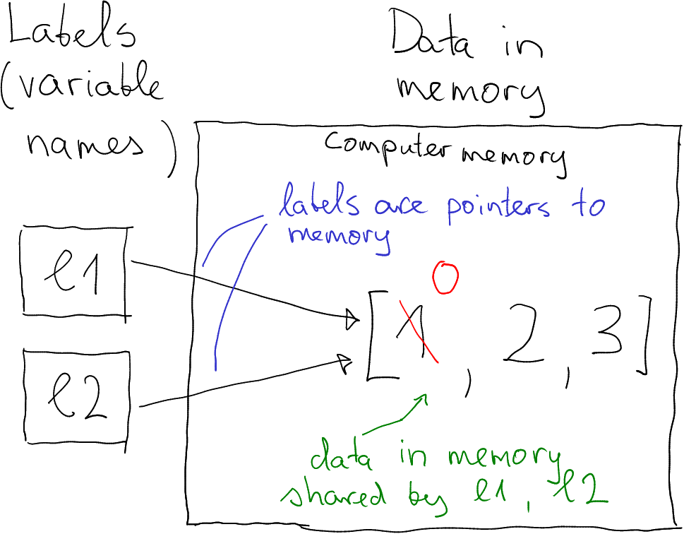
Two objects (l1 and l2) share the same memory.
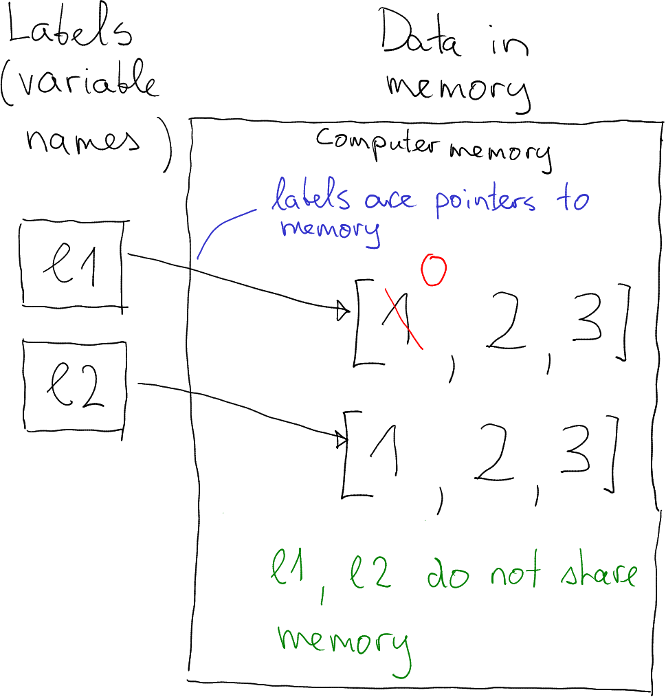
In order to understand what is going on here, we need to understand what are the variables, here complex variables like lists. While you can imagine that simple variables (like numbers or strings) are just boxes that contain the value, this is not true for lists and for other more complex objects. Instead, the variable name is basically a label that points to a location in computer memory where the data is stored (see the figure).
Now when you create l2 as l2 = l1, then you do
not copy the data in memory! We are copying l1 to l2 but at the
same time we are not copying the underlying data structure. This is
called shallow copy. You just create another label that
points to the same location!
Thereafter, when we modify l1 and replace the first element with
“0”, the modification occurs in the memory, in the same location that
both lists point to. Hence both of them will now point to a modified
data structure where the first element is “0”.
This approach as clear advantages (see below), but it is not always
what you want. Fortunately, you can explicitly request a copy with
.copy() method:
## [1, 2, 3]Here the .copy() method makes a deep copy of the
list–duplicates the data in memory. Now modification of l1 does
not affect l2. The lists do not share any memory.
What are the advantages of in-place operations? The main advantage is faster speed and lower memory requirements. The memory side is fairly obvious–if you perform a shallow copy, then you just keep a single copy of data in memory. And the origin of speed difference is the same–performing a deep copy of large data structures is slow.
Unlike python, R does not modify objects in place, but always makes a deep copy when you modify an object. This may make R code very slow if you are modifying huge matrices element-by-element. Each time you modify a single element, R makes a copy of the whole matrix.
In-place operations have two major disadvantages. First, they are more complex. You need to understand that they exist, and which kind of data structures they are used for. Python has a plethora of methods that perform operations in place, that return a modified copy, or where you can specify what do you want. This may be overwhelming for people with little coding background. Second potential problem are sneaky bugs that may happen if you are not careful enough. In R, functions will never modify their argument. In python this is possible, and may cause hard-to-find errors.
Typically, the advantages outweigh the disadvantages for experienced coders and larger datasets, and the way around.
2.5.2 Methods that return and methods that modify
Many functions return the object, many methods modify the object (and return nothing), while certain methods allow you to choose what to do. This may be a bit overwhelming for the beginners. As a reminder, method is a “property” of objects, certain kind of “appendix”-functions of the objects that operate on that object.
Here is an example of method that returns a modified object:
## 'TEXT'## 'text'However, there are plenty of methods that modify the objects. This
includes sorting the list, .sort() methods orders the elements in a
natural order:
## [1, 2, 3, 5]So .sort()
operates in place and modifies the current list, unlike .upper().
This is a frequent source of confusion and errors,
for instance if you forget about sort working in-place, you may
mistakenly write
l1 is empty.
However, there is a function sorted that returns a sorted list
while leaving the original list untouched:
## [1, 2, 3, 5]## [1, 5, 3, 2]Presence of similar functions, some which work in place and some of which return a modified object is a frequent source of confusion for beginners. Unlike python, R avoids such confusion by always returning a modified value. This is good for beginners, but grossly inefficient when working with large datasets.
2.6 Language Constructs
2.6.1 if-elif-else
if-construct works in a very predictable manner, in a similar
fashion as in many other common languages:
if requires a logical expression. If this is true, the following
indented block is executed. If it is not true, the eventual elif
condition is checked (there may be many elif-blocks), and finally else block is executed given there
is an else-block.
Sometimes it is useful to have a block that does nothing. In that
case on may use pass-statement:
Note that it is usually better to invert the logical condition and leave out the else block instead.
2.6.2 for-Loops
For loops are one of the favorite ways of iterating over collections.
The only requirement is the collection to be iterable, it does not
have to be ordered (and even more, it does not to be a collection,
like range is not a collection. The syntax is easy to remember:
for _variable_ in _collection_:. The colon is followed by an
indented block, the body of the for loop.
A trivial example:
## 0
## 1
## 2
Remember that the collection does not to contain elements of the same type. We can also do
## 1
## a
## True
And finally an example of functional programming: we loop over a list of functions, and print the function value at 1:
## 0.8414709848078965
## 0.5403023058681398
## 1.0
import is the python way to load libraries (modules), see Modules.
Exercise 2.10 For numbers 1 to 10, print out their parity (odd or even). Proceed as follows:
- Loop over numbers 1 to 10
- Use the modulo operator
%to check if the number is odd (the number modulo 2 is 1) or even. - use if/else to print the number, and the corresponding parity. The output should look like:
1 odd
2 even
...
See the solution
For-loops is a handy tool for various tasks. Quite often we need to calculate something based on a number of items. In that case we want to initialize the result (also called accumulator), and update it in a for loop where we iterate over all these items. For instance, we can use for-loops to compute factorials (product of all integers up to a given number):
## 3628800And here is another example: combine all names in a list so we have a single, comma-separated string:
## flowers
names = ["viola glabella", "monothropa hypopithys", "lomatium utriculatum"]
s = ""  # initialize accumulator
for name in names:
    if s != "":
        s += ", "
    s += name
s
## 'viola glabella, monothropa hypopithys, lomatium utriculatum'Here the code needs to work slightly differently, depending on if we
are working with the first or with a subsequent name, as only the
subsequent ones are preceded by ", ".
These examples above are trivial, and there are easier ways to achieve the results using standard python libraries. But this approach is more general and can be applied in many cases where no such library functions exist.
Exercise 2.11 Do the second task, combining names into a long comma-separated
list, using the string .join() method.
See the solution
2.7 Libraries (modules)
Base python automatically loads a minimalistic set of functions. For instance, it does not load common mathematical operators like square root or sinus, and it does not load operating system functionality like directory listings. Such functionality must be loaded explicitly by importing the corresponding modules (libraries).
There are different ways to import modules. First, one can load the
whole module, and use the syntax module-name.function to access the
function. For instance:
## 1.4142135623730951This imports the math module that contains a plethora of
mathematical operations, and afterwards we can use these functions
with math. prefix. The advantage of this approach is that in code one can
immediately see where are certain functions coming from. However, it
involves more typing and longer names.
Alternatively, we can only import the necessary functions, and use those without the prefix:
## 1.4142135623730951## 1.0This results in shorter and cleaner code, but sometimes it may be hard
to guess where are the corresponding functions defined. Function
sin may be defined either in the math module, numpy module, or
maybe just elsewhere in the same code file.
It is also possible to rename the module when importing, a very popular approach when working with libraries with longer names:
## 1.4142135623730951## 1.0Exercise 2.12 Access your file system. File system functions are not loaded by
default, but they reside in the os module.
Find your working directory, and list files therein. Use functions
getcwd (get current working directory) and listdir in that
module.
See the solution
In principle on can also compute hash code of mutable variables. However, that would require computer to be aware of any data changes, and if that happens the recompute the hash code. It is doable, but inefficient. Python solves this dilemma in a way that it only computes hash codes for immutable variables.↩︎