Chapter 15 Regularization and Feature Selection

This section discusses a very common ML issue: you have too many features, and you do not know which ones to include. There are many ways to do feature selection, below we discuss a few more popular ones.

We assume you have loaded the following packages:

import numpy as np
import pandas as pd
import matplotlib.pyplot as plt

Below we load more as we introduce more.

For replicability, we also set the seed:

np.random.seed(1)

15.1 How highly correlated features fail

correlated-data is a small dataset that contains a number of highly correlated features. This allows to demonstrate the problem in a small scale:

df = pd.read_csv(
    "../../../tyyq/teaching/data/toy/correlated-data.csv.bz2",
    sep = "\t")

The dataset contains the outcome y and 40 features, labeled as x1–x20 and z1–z20:

df.shape

## (100, 41)

df.columns

## Index(['y', 'x1', 'x2', 'x3', 'x4', 'x5', 'x6', 'x7', 'x8', 'x9', 'x10', 'x11',
##        'x12', 'x13', 'x14', 'x15', 'x16', 'x17', 'x18', 'x19', 'x20', 'z1',
##        'z2', 'z3', 'z4', 'z5', 'z6', 'z7', 'z8', 'z9', 'z10', 'z11', 'z12',
##        'z13', 'z14', 'z15', 'z16', 'z17', 'z18', 'z19', 'z20'],
##       dtype='object')

the x-features are highly correlated numbers and z-features are highly correlated letters. Here a small sample:

df[["y", "x1", "x2", "x3", "z1", "z2", "z3"]].sample(4)

##            y        x1        x2        x3 z1 z2 z3
## 80  2.910576  1.136508  1.551260  1.123826  B  B  B
## 84 -0.857186  1.403782  2.671632  1.411380  C  C  C
## 33 -0.267300 -0.727276 -0.310559 -0.730979  A  A  A
## 81  3.297370  0.806009  0.919699  0.800474  A  A  A

I convert the letters to dummies and separate a small (40 cases) validation set from the data:

from sklearn.model_selection import train_test_split

y = df.y
X = df.drop("y", axis = 1)
X = pd.get_dummies(X, drop_first = True)
Xt, Xv, yt, yv = train_test_split(X, y, test_size = 0.4,
                                  random_state = 8)
Xt.shape

## (60, 60)

So the design matrix we work with now contains 60 columns and 60 rows. Below, we’ll work with Xt and yt and leave Xv and yv for validation.

As a first step, lets fit a linear regression model on all the features and compute \(R^2\), both on training and validation data:

from sklearn.linear_model import LinearRegression

m = LinearRegression()
_t = m.fit(Xt, yt)
m.score(Xt, yt)

## 0.9677374023461163

m.score(Xv, yv)

## 0.8521445384390035

This suggests a substantial overfitting: training \(R^2\) is noticeably larger than validation \(R^2\).

15.2 Forward selection

There are several solutions to this problem. A popular algorithm is forward selection where one first picks the best 1-feature model, thereafter tries adding all remaining features one-by-one to build the best two-feature model, and thereafter the best three-feature model, and so on, until the model performance starts to deteriorate.

0-feature base model:

m0 = LinearRegression(fit_intercept = False)
X0 = np.ones((X.shape[0], 1))
X0t, X0v, yt, yv = train_test_split(X0, y, test_size = 0.4,
                                    random_state = 8)
_t = m0.fit(X0t, yt)
m0.score(X0v, yv)

## -0.006849647990198937

Try 1-feature models:

best1 = {"i": -1, "R2": -np.inf}
m1 = LinearRegression(fit_intercept = True)
for i in range(X.shape[1]):
    X1 = X.iloc[:,[i]]
    X1t, X1v, yt, yv = train_test_split(X1, y, test_size = 0.4,
                                    random_state = 8)
    _t = m1.fit(X1t, yt)
    s = m1.score(X1v, yv)
    if s > best1["R2"]:
        best1["i"] = i
        best1["R2"] = s
        
best1

## {'i': 9, 'R2': 0.4666428183761875}

Add another feature:

best2 = {"i": -1, "R2": -np.inf}
m2 = LinearRegression(fit_intercept = True)
included_features = set([best1["i"]])
features_to_test = set(range(X.shape[1])) - included_features
for f in features_to_test:
    features = included_features.union({f})
    X2 = X.iloc[:, list(features)]
    X2t, X2v, yt, yv = train_test_split(X2, y, test_size = 0.4,
                                    random_state = 8)
    _t = m2.fit(X2t, yt)
    s = m2.score(X2v, yv)
    if s > best2["R2"]:
        best2["i"] = f
        best2["R2"] = s
        
best2

## {'i': 2, 'R2': 0.8677935861014889}

Can add more in this fashion.

Make a function:

def bestFeature(X, y, included_features):
    best = {"i": -1, "R2": -np.inf}
    features_to_test = list(
        set(range(X.shape[1])) - set(included_features))
    for f in features_to_test:
        features = included_features + [f]
        Xf = X.iloc[:, features]
        Xft, Xfv, yt, yv = train_test_split(Xf, y, test_size = 0.4,
                                            random_state = 8)
        _t = m2.fit(Xft, yt)
        s = m2.score(Xfv, yv)
        if s > best["R2"]:
            best["i"] = f
            best["R2"] = s
    return best

best = list()
included_features = []
r2s = []
for f in range(X.shape[1]):
    b = bestFeature(X, y, included_features)
    best.append(b)
    included_features = included_features + [b["i"]]
    r2s.append(b["R2"])
best

## [{'i': 9, 'R2': 0.4666428183761875}, {'i': 2, 'R2': 0.8677935861014889}, {'i': 27, 'R2': 0.9296522813032738}, {'i': 28, 'R2': 0.9396723227644169}, {'i': 14, 'R2': 0.9430611422142999}, {'i': 22, 'R2': 0.9437993501430609}, {'i': 33, 'R2': 0.9446022123630593}, {'i': 59, 'R2': 0.9450369454683459}, {'i': 10, 'R2': 0.9452498568205782}, {'i': 8, 'R2': 0.9455986815032276}, {'i': 19, 'R2': 0.946286246742816}, {'i': 1, 'R2': 0.9464320773146166}, {'i': 46, 'R2': 0.9465914853888852}, {'i': 40, 'R2': 0.9465889082229212}, {'i': 55, 'R2': 0.9465359196145451}, {'i': 36, 'R2': 0.9464542982901596}, {'i': 5, 'R2': 0.9463762822853349}, {'i': 20, 'R2': 0.9462833979835925}, {'i': 34, 'R2': 0.9462050456158059}, {'i': 48, 'R2': 0.9461478229257212}, {'i': 50, 'R2': 0.9461054197700753}, {'i': 52, 'R2': 0.9460730478692244}, {'i': 26, 'R2': 0.9459904691472556}, {'i': 42, 'R2': 0.9459265694540919}, {'i': 44, 'R2': 0.9458087497124463}, {'i': 32, 'R2': 0.9455590142220007}, {'i': 39, 'R2': 0.9454085021414114}, {'i': 25, 'R2': 0.9449675269753557}, {'i': 24, 'R2': 0.944534691438683}, {'i': 58, 'R2': 0.943866554555072}, {'i': 54, 'R2': 0.9431161004717257}, {'i': 38, 'R2': 0.9425908604390919}, {'i': 21, 'R2': 0.9418808150038424}, {'i': 35, 'R2': 0.9414073375383594}, {'i': 37, 'R2': 0.9410776069690766}, {'i': 41, 'R2': 0.9408366363995861}, {'i': 49, 'R2': 0.9406534112839532}, {'i': 51, 'R2': 0.940509615245991}, {'i': 53, 'R2': 0.9403938540834736}, {'i': 43, 'R2': 0.9401119255355866}, {'i': 57, 'R2': 0.9397885757150685}, {'i': 23, 'R2': 0.9394085387576047}, {'i': 12, 'R2': 0.9379313435724344}, {'i': 30, 'R2': 0.9377835490332774}, {'i': 45, 'R2': 0.9333091167915861}, {'i': 29, 'R2': 0.9340676090843352}, {'i': 16, 'R2': 0.9285874234675197}, {'i': 0, 'R2': 0.9182942310440995}, {'i': 11, 'R2': 0.9182942310438696}, {'i': 18, 'R2': 0.9182942310438482}, {'i': 15, 'R2': 0.9182942310437175}, {'i': 3, 'R2': 0.9182942310436977}, {'i': 13, 'R2': 0.918294231043749}, {'i': 4, 'R2': 0.9182942310436918}, {'i': 17, 'R2': 0.9182942310436858}, {'i': 6, 'R2': 0.8808093695322948}, {'i': 7, 'R2': 0.8808093695322833}, {'i': 56, 'R2': 0.8437760019668595}, {'i': 31, 'R2': 0.8474899063074901}, {'i': 47, 'R2': 0.8521445384389958}]

plt.s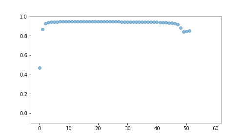catter(range(len(r2s)), r2s, alpha = 0.5)
plt.ylim(-0.1, 1)

## (-0.1, 1.0)

plot of chunk unnamed-chunk-12

from sklearn.feature_selection import SequentialFeatureSelector

m = LinearRegression()
sfs = SequentialFeatureSelector(m)
_t = sfs.fit(Xt, yt)
sfs.get_feature_names_out()

## array(['x3', 'x10', 'z1_B', 'z1_C', 'z2_B', 'z2_C', 'z4_B', 'z4_C',
##        'z5_B', 'z6_B', 'z7_B', 'z7_C', 'z8_B', 'z8_C', 'z10_B', 'z10_C',
##        'z11_C', 'z12_B', 'z13_B', 'z13_C', 'z14_B', 'z14_C', 'z15_B',
##        'z16_B', 'z17_B', 'z18_B', 'z18_C', 'z19_B', 'z20_B', 'z20_C'],
##       dtype=object)

Xtr = sfs.transform(Xt)
Xvr = sfs.transform(Xv)
_t = m.fit(Xtr, yt)
m.score(Xvr, yv)

## 0.9331571645766498

15.3 Ridge and Lasso regression

Ridge and Lasso are methods that are related to forward selection. These methods penalize large \(\beta\) values and hence suppress or eliminate correlated variables. These do not need looping over different combinations of variables like forward selection, however, one normally has to loop over the penalty parameter alpha to find the optimal value.

Both methods are living in sklearn.linear_regression. We demonstrate this with ridge regression below:

from sklearn.linear_model import Ridge, Lasso
from sklearn.model_selection import cross_val_score

m = Ridge(alpha = 1)  # penalty value 1
cross_val_score(m, X, y, cv=10).mean()

## np.float64(0.908232518044392)

m = Ridge(alpha = 0.3)  # penalty value 0.1
cross_val_score(m, X, y, cv=10).mean()

## np.float64(0.9035580051705517)

As evident from the above, penalty values 1 and 0.3 give virtually equal results. The cross-validated \(R^2\) is also comparable to what forward-selection suggested.

Lasso works in an analogous fashion as ridge, but as it’s penalty is not globally differentiable (it is \(L_1\) penalty), then you may run into more problems with convergence.

Both methods have more options, in particular they can normalize the features before fitting.

m = Ridge(alpha = 1)
_t = m.fit(Xt, yt)
m.score(Xv, yv)

## 0.9264571331356263

m = Lasso(alpha = 1)
_t = m.fit(Xt, yt)
m.score(Xv, yv)

## 0.8627943726880424