Chapter 20 Machine learning technicques

I assume you have loaded the following modules:

import numpy as np
import matplotlib.pyplot as plt

20.1 Gradient descent

20.1.1 Vector functions

We call functions that either accept a vector argument, or return a vector results (or both) as vector functions. Vector functions can be defined and used in almost the same way that “ordinary” scalar functions. For instance, here a function that adds two vectors:

def add(v1, v2):
    v = v1 + v2
    return v

This is a vector function in a sense that both it arguments and value are vectors (as written above, the arguments don’t even have to be vectors, just numbers and even strings will do). You can use this function as

x = np.array([1, 2, 3])
y = np.array([10, 20, 30])
add(x, y)

## array([11, 22, 33])

While this is a valid function, it is not particularly useful as just the “+” operator achieves exactly the same. Let’s compute the Euclidan norm of a vector, \(||\boldsymbol{x}|| = \sqrt{\boldsymbol{x}' \cdot \boldsymbol{x}}\) using the \(\boldsymbol{x}\) from above:

def norm(x):
    n = np.sqrt(x.T @ x)
    return n

norm(x)

## 3.7416573867739413

This function uses dedicated vector operations–.T and @–and returns a single number. As both of these are dimension-independent, the function will work with vectors of any dimension. It return a scalar, so it is a vector-argument, scalar-valued function.

The gradient of this function is \(f(\boldsymbol{x}) = 2 \boldsymbol{x}\). This is a vector-argument-vector-valued function. You can implement it in python as:

def grad(x):
    return 2*x

grad(x)

## array([2, 4, 6])

grad(y)

## array([20, 40, 60])

So vector functions are the same as the as normal functions when you write the code. Just arguments and return values are vectors.

Exercise 20.1

Consider a function \(f(\boldsymbol{x}) = e^{-\boldsymbol{x}' \cdot \boldsymbol{x}}\) where \(\boldsymbol{x}' = (x_{1}, x_{2})\).

Define the function in python. It’s argument should be a single vector \(\boldsymbol{x}\), and it should do the calculations in vector form.
Compute the function value at \(\boldsymbol{x}_1 = (0, 1)'\), \(\boldsymbol{x}_2 = (1, 0)'\) and \(\boldsymbol{x}_3 = (1, 1)'\). Use column vectors as input!
Compute (analytically, on paper) the gradient of the function. You may want to do it in non-vector form, writing the function as \(f(x_{1}, x_{2}) = e^{-(x_{1}^{2} + x_{2}^{2})}\). Compute the gradient, and transform it back into vector form!
Define the gradient function in python. It should have a single argument, the vector \(\boldsymbol{x}\), and it should return a vector, the gradient value.
Use the function to compute the gradient value at \(\boldsymbol{x}_{1} = (0, 1)'\), \(\boldsymbol{x}_{2} = (1, 0)'\) and \(\boldsymbol{x}_{3} = (1, 1)'\).
Can this function compute gradient value at \(\boldsymbol{x}_{1} = (0, 1, 2, 3)'\)? Explain, and try!

The solution

When implementing a quadratic form, e.g. \(\boldsymbol{x}` \mathsf{A} \boldsymbol{x}\), you can either supply \(\mathsf{A}\) as an argument, as an argument with a default value, or define it as a global value. So all these methods will do:

## A as regular argument
def qf(x, A):
    q = x.T @ A @ x
    return q

A = np.eye(2)
x = np.array([1, 2])
qf(x, A)

## 5.0

## Regular argument with a default value
def qf1(x, A = np.eye(2)):
    q = x.T @ A @ x
    return q

qf1(x)

## 5.0

## Global variable
B = np.eye(2)
def qf2(x):
    q = x.T @ B @ x
    return q

qf2(x)

## 5.0

Which one to use depends on how do you want to treat the “parameter” argument \(\mathsf{A}\). But you may want to add some extra code to ensure \(\mathsf{A}\) and \(\boldsymbol{x}\) are compatible.

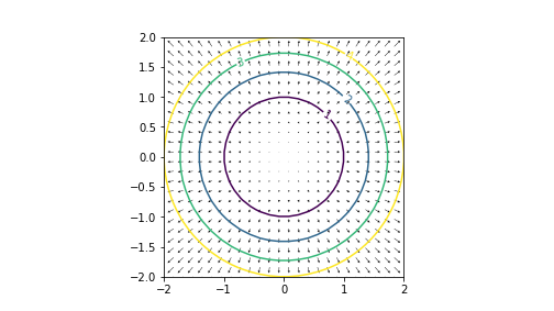
20.1.2 Visualizing the function and gradient

It is only meaningful to visualize functions of a 2-D vector argument, and those that return a 2-D vector value. In higher dimensions the visualization will not really work, and in 1-D case it is quite simplistic. Let’s do it with the simple quadratic form \(\boldsymbol{x}' \boldsymbol{x}\) (its gradient is \(2 \boldsymbol{x}\)). First define the function and its gradient:

def f(x):
    z = x.T @ x
    return z

def grad(x):
    g = 2 * x
    return g

Next, here is code that visualizes both the function and the gradient. It calculates the function and the gradient on a grid, visualizes the former as a contour plot, overlaid with arrows for the gradient:

def showFG(f,  # function: must work with a single 2-D vector argument
           grad = None,  # gradient.
           # Must accept the same argument as function
           # must return a 2-D vector
           levels = (1, 2, 3, 4),
           # contour levels to be drawn
           x1range = (-2, 2), x2range=(-2, 2),
           # range over which to make the plot
           nGrid = 26  # the grid density where to compute 
           ):
    ## Make the grid
    ex1 = np.linspace(x1range[0], x1range[1], nGrid)
    ex2 = np.linspace(x2range[0], x2range[1], nGrid)
    (xm1, xm2) = np.meshgrid(ex1, ex2)
    x1 = xm1.ravel()
    x2 = xm2.ravel()
    ## Initialize the function and gradient matrices
    z = np.zeros_like(xm1)  # function values
    g1 = np.zeros_like(xm1)  # first component of the gradient
    g2 = np.zeros_like(xm1)  # second component
    ## Compute function/grandient on the grid in a loop
    for i in range(nGrid):
        for j in range(nGrid):
            x = np.array([[xm1[i,j]], [xm2[i,j]]])
            z[i,j] = f(x)[0,0]
            if grad is not None:
               g = grad(x)
               g1[i,j] = g[0,0]
               g2[i,j] = g[1,0]
    ## Plot the function using contours
    fig = plt.figure()
    ax = fig.add_subplot(111)
    ax.set_aspect('equal')
    cs = ax.contour(ex1, ex2, z, levels = levels)
    ax.clabel(cs, inline=1, fontsize=10)
    ## Add arrows
    ax.quiver(ex1, ex2, g1, g2, width=0.002, headwidth=5)
    ## Print suggested levels, in case you don't know what
    ## are good values
    print("Suggested levels:")
    print(np.percentile(z, (20, 40, 60, 80)))

Finally, make the plot:

showFG(f, grad)

It shows a 2-D parabola with its focus (the minimum) at \((0, 0)\).