A Solutions
## /home/otoomet/R/x86_64-pc-linux-gnu-library/4.5/reticulate/python/rpytools/loader.py:120: UserWarning: Pandas requires version '1.3.6' or newer of 'bottleneck' (version '1.3.5' currently installed).
##   return _find_and_load(name, import_)
A.1 Python
A.1.1 Operators
A.1.3 Collections
A.1.3.2 Combining lists
friends = ['Paulina', 'Severo']
others = []
others.append("Lai Ming")
others.append("Lynn")
people = friends + others
print("all people", people)
## all people ['Paulina', 'Severo', 'Lai Ming', 'Lynn']A.1.3.3 Assign people to seats
Consider two lists:
names = ["Adam", "Ashin", "Inukai", "Tanaka", "Ikki"]
seats = [33, 12, 45, 2, 17]
assigneds = []
for i in range(len(names)):
    a = names[i] + ": " + str(seats[i])
    assigneds.append(a)
assigneds
## ['Adam: 33', 'Ashin: 12', 'Inukai: 45', 'Tanaka: 2', 'Ikki: 17']A.1.3.4 List comprehension
- make list of not
ibut ofi + 1:
## [1, 2, 3, 4, 5, 6, 7, 8, 9, 10]- To make pizzas with different toppings you can just
use string concatenation with
+:
## ['pizza with mushrooms', 'pizza with mozarella', 'pizza with ananas']- Here you can just loop over the lists, and each time pick out
element
[1]from the list:
## [2, 'b', <built-in function print>]A.1.3.5 Dict mapping coordinates to cities
placenames = {(31.228611, 121.474722): "Shanghai",
              (23.763889, 90.388889): "Dhaka",
              (13.7525, 100.494167): "Bangkok"
          }
print(placenames)
## {(31.228611, 121.474722): 'Shanghai', (23.763889, 90.388889): 'Dhaka', (13.7525, 100.494167): 'Bangkok'}Note that such lookup is usually not what we want because it only returns the correct city name if given the exact coordinates. If coordinates are just a tiny bit off, the dict cannot find the city. If you consider cities to be continuous areas, you should do geographic lookup, not dictionary lookup.
A.1.3.6 Dict of dicts
tsinghua = {"house":30, "street":"Shuangqing Rd",
            "district":"Haidan", "city":"Beijing",
            "country":"CH"}
kenyatta = {"pobox":"43844-00100", "city":"Nairobi",
            "country":"KE"}
places = {"Tsinghua":tsinghua, "Kenyatta":kenyatta}
places["Teski Refugio"] = {"house":256,
                   "street":"Volcan Osorno",
                   "city":"La Ensenada",
                   "region":"Los Lagos",
                   "country":"CL"}
print(places)
## {'Tsinghua': {'house': 30, 'street': 'Shuangqing Rd', 'district': 'Haidan', 'city': 'Beijing', 'country': 'CH'}, 'Kenyatta': {'pobox': '43844-00100', 'city': 'Nairobi', 'country': 'KE'}, 'Teski Refugio': {'house': 256, 'street': 'Volcan Osorno', 'city': 'La Ensenada', 'region': 'Los Lagos', 'country': 'CL'}}A.1.4 Language Constructs
A.1.4.1 Solution: odd or even
## 1 odd
## 2 even
## 3 odd
## 4 even
## 5 odd
## 6 even
## 7 odd
## 8 even
## 9 odd
## 10 evenA.1.5 Modules
A.1.5.1 Solution: access your file system
Below is the solution by importing the whole libraries. You can also
use, e.g. from os import getcwd, listdir, or other approaches.
## '/home/otoomet/tyyq/lecturenotes/machinelearning-py'## ['solutions.md', 'index.md', 'images.rmd', 'Makefile', 'neural-nets.rmd', 'ml-techniques.rmd~', 'python.rmd', 'neural-nets.md', 'web-scraping.rmd', 'ml-workflow.md', 'text.rmd', 'descriptive-statistics.rmd', 'python.md', 'titanic-tree.png', 'predictions.md', 'solutions.rmd', '_bookdown.yml', 'datasets.md', 'descriptive-statistics.md', 'ml-techniques.md', 'index.rmd', 'predictions.rmd', 'build', 'trees-forests.md', '.cache', 'regularization.rmd', 'trees-forests.rmd', 'unsupervised-learning.md', 'images.md', 'linear-regression.rmd', 'overfitting-validation.rmd', 'web-scraping.md', 'torch-color-spiral.py~', 'linear-algebra.md', 'linear-algebra.rmd', 'keras-cats-vs-dogs.py', 'svm.md', 'svm.rmd', 'overfitting-validation.md', 'cleaning-data.md', 'numpy-pandas.rmd', 'plotting.rmd', '_output.yml', 'figs', 'logistic-regression.rmd', 'keras-color-spiral.py', 'descriptive-analysis.rmd', 'ml-techniques.rmd', 'linear-regression.md', 'cleaning-data.rmd', 'ml-workflow.rmd', 'torch-color-spiral.py', 'unsupervised-learning.rmd', 'img', 'numpy-pandas.md', 'logistic-regression.md', 'files', 'descriptive-analysis.md', 'text.md', 'datasets.rmd', 'machinelearning-py.rds', '.fig', 'regularization.md', 'plotting.md']A.2 Numpy and Pandas
A.2.1 Numpy
A.2.1.1 Solution: concatenate arrays
## array([[-1., -1., -1., -1.],
##        [ 0.,  0.,  0.,  0.],
##        [ 2.,  2.,  2.,  2.]])
Obviously, you can use np.ones and np.zeros directly in
np.row_stack and skip creating the temporary variables.
A.2.1.2 Solution: create matrix of even numbers
## array([[ 2,  4,  6,  8, 10],
##        [12, 14, 16, 18, 20],
##        [22, 24, 26, 28, 30],
##        [32, 34, 36, 38, 40]])
A.2.1.3 Solution: create matrix, play with columns
## [14 24 34 44]## array([[10, 12, 14, 16, 18],
## [20, 22, 24, 26, 28],
## [30, 32, 34, 36, 38],
## [ 1, 2, 3, 4, 5]])A.2.2 Pandas
A.2.2.1 Solution: series of capital cities
cities = pd.Series(["Brazzaville", "Libreville", "Malabo", "Yaoundé"],
                   index=["Congo", "Gabon", "Equatorial Guinea", "Cameroon"])
cities
## Congo Brazzaville
## Gabon Libreville
## Equatorial Guinea Malabo
## Cameroon Yaoundé
## dtype: objectA.2.2.2 Solution: extract capital cities
## 'Brazzaville'## 'Malabo'## Gabon Libreville
## dtype: objectA.2.2.3 Solution: create city dataframe
To keep code clean, we create data as a separate dict, and index as a list. Thereafter we make a dataframe out of these two:
data = {"capital":["Brazzaville", "Libreville", "Malabo", "Yaoundé"],
        "population":[1696, 703, 297, 2765]}
countries = ["Congo", "Gabon", "Equatorial Guinea", "Cameroon"]
cityDF = pd.DataFrame(data, index=countries)
cityDF
## capital population
## Congo Brazzaville 1696
## Gabon Libreville 703
## Equatorial Guinea Malabo 297
## Cameroon Yaoundé 2765A.2.2.4 Solution: Variables in G.W.Bush approval data frame
Pandas prints five columns: index, and four variables— date, approve, disapprove, dontknow.
A.2.2.5 Show files in current/parent folder
Remember that parent folder is denoted as double dots ... Current
folder is a single dot ., but usually it is not needed.
Current working directory:
## '/home/otoomet/tyyq/lecturenotes/machinelearning-py'Files in the current folder
## ['solutions.md', 'index.md', 'images.rmd', 'Makefile', 'neural-nets.rmd', 'ml-techniques.rmd~', 'python.rmd', 'neural-nets.md', 'web-scraping.rmd', 'ml-workflow.md', 'text.rmd', 'descriptive-statistics.rmd', 'python.md', 'titanic-tree.png', 'predictions.md', 'solutions.rmd', '_bookdown.yml', 'datasets.md', 'descriptive-statistics.md', 'ml-techniques.md', 'index.rmd', 'predictions.rmd', 'build', 'trees-forests.md', '.cache', 'regularization.rmd', 'trees-forests.rmd', 'unsupervised-learning.md', 'images.md', 'linear-regression.rmd', 'overfitting-validation.rmd', 'web-scraping.md', 'torch-color-spiral.py~', 'linear-algebra.md', 'linear-algebra.rmd', 'keras-cats-vs-dogs.py', 'svm.md', 'svm.rmd', 'overfitting-validation.md', 'cleaning-data.md', 'numpy-pandas.rmd', 'plotting.rmd', '_output.yml', 'figs', 'logistic-regression.rmd', 'keras-color-spiral.py', 'descriptive-analysis.rmd', 'ml-techniques.rmd', 'linear-regression.md', 'cleaning-data.rmd', 'ml-workflow.rmd', 'torch-color-spiral.py', 'unsupervised-learning.rmd', 'img', 'numpy-pandas.md', 'logistic-regression.md', 'files', 'descriptive-analysis.md', 'text.md', 'datasets.rmd', 'machinelearning-py.rds', '.fig', 'regularization.md', 'plotting.md']Files in the parent folder
## ['machineLearning.mtc3', 'machineLearning.mtc17', 'machineLearning.mtc8', 'machineLearning.mtc2', 'data', 'Makefile', 'machineLearning.pdf', 'machineLearning.mtc14', 'machineLearning.mtc20', 'lecturenotes.bib.bak', 'machinelearning-R.html', 'machineLearning.mtc10', 'latexmkrc', 'tex', 'auto', '.RData', 'machineLearning.mtc9', 'preamble.tex', 'scripts', 'machineLearning.mtc18', 'machineLearning.exc', 'machineLearning.mtc13', 'intro-to-stats.rnw', 'machineLearning.mtc21', 'machineLearning.mtc19', 'machineLearning.mtc16', 'machineLearning.mtc5', '.cache', 'material', 'machineLearning.tex', 'solutions.rnw', 'machineLearning.maf', 'machineLearning.mtc0', 'machineLearning.mtc11', 'ml-models.rnw', 'machineLearning.mtc12', 'machinelearning-py', 'kbordermatrix.sty', 'machinelearning-R', 'solutions.tex', 'datascience-intro', 'machinelearning-common', 'machineLearning.chs', 'test', 'machineLearning.mtc1', 'machineLearning.exm', 'machineLearning.mtc23', 'machineLearning.mtc15', 'figs', 'machineLearning.mtc7', '.Rprofile', '.git', 'intro-to-stats.tex', 'machineLearning.mtc4', 'machineLearning.rnw', 'img', 'machineLearning.mtc', 'machineLearning.bbl', 'README.md', 'files', 'machineLearning.mtc22', '.Rhistory', 'solutions.tex~', 'videos', '.gitignore', 'machineLearning.rip', '.fig', 'machineLearning.tex~', 'ml-models.tex', 'literature', 'machineLearning.mtc6']Obviously, everyone has different files in these folders.
A.2.2.6 Solution: presidents approval 88%
approval = pd.read_csv("../data/gwbush-approval.csv", sep="\t", nrows=10)
approval[approval.approve >= 88][["date", "approve"]]  # only print date,
## date approve
## 5 2001 Oct 19-21 88
## 6 2001 Oct 11-14 89
## 8 2001 Sep 21-22 90## 3A.2.2.7 Solution: change index, convert to variable
The original data frame was created as
capitals = pd.DataFrame(
        {"capital":["Kuala Lumpur", "Jakarta", "Phnom Penh"],
         "population":[32.7, 267.7, 15.3]},  # in millions
        index=["MY", "ID", "KH"])
We can modify it as
##                 capital  population
## Malaysia   Kuala Lumpur        32.7
## Indonesia       Jakarta       267.7
## Cambodia Phnom Penh 15.3A.2.2.8 Solution: create city dataframe
cityM = np.array([[3.11, 5282, 19800],
              [18.9, 306, 46997],
              [4.497, 1886, 22000]])
names = ["Chittagong", "Dhaka", "Kolkata"]
vars = ["population", "area", "density"]
cityDF = pd.DataFrame(cityM, index=names,
                      columns=vars)
cityDF
## population area density
## Chittagong 3.110 5282.0 19800.0
## Dhaka 18.900 306.0 46997.0
## Kolkata 4.497 1886.0 22000.0A.2.2.9 Solution: extract city data
## array([19800., 46997., 22000.])## Chittagong 19800.0
## Dhaka 46997.0
## Kolkata 22000.0
## Name: density, dtype: float64## array([4.497e+00, 1.886e+03, 2.200e+04])## population 4.497
## area 1886.000
## density 22000.000
## Name: Kolkata, dtype: float64## population 4.497
## area 1886.000
## density 22000.000
## Name: Kolkata, dtype: float64## 306.0## 1886.0## 306.0A.2.2.10 Solution: Titanic line 1000
Extract the 1000th row (note: index 999!) as data frame, and thereafter extract name, survival status, and age. We have to extract twice as we cannot extract by row number and column names at the same time.
##                                   name  survived  age
## 999  McCarthy, Miss. Catherine "Katie"         1  NaN
A.2.2.11 Solution: Titanic male/female age distribution
The two relevant variables are clearly sex and age. If you already have loaded data then you may just presereve these variables:
##         sex   age
## 934  female   4.0
## 4    female  25.0
## 827    male  11.0
## 475  female  26.0
Alternatively, you may also just read these two columns only:
##       sex   age
## 547  male  23.0
## 240  male  45.0
## 140  male  23.0
## 900  male   NaN
A.3 Descriptive analysis with Pandas
A.3.1 What are the values?
A.3.1.1 Solution: which methods can be applied to the whole data frame
There is no better way than just to try:
## TypeError: '<=' not supported between instances of 'str' and 'float'## TypeError: can only concatenate str (not "int") to str## AttributeError: 'DataFrame' object has no attribute 'unique'. Did you mean: 'nunique'?## pclass 3
## survived 2
## name 1307
## sex 2
## age 98
## sibsp 7
## parch 8
## ticket 929
## fare 281
## cabin 186
## embarked 3
## boat 27
## body 121
## home.dest 369
## dtype: int64The mathematical functions work, but may skip the non-numeric
variables. .min however, find the first value when ordered
alphabetically.
It is not immediately clear why .unique does not work while
.nunique works. It may be because there is a different number of
unique elements for each variables, but hey, you can just use a more
complex data structure and still compute that.
A.4 Cleaning and Manipulating Data
A.4.1 Missing Observations
A.4.1.1 Solution: Missings in fare in Titanic Data
We can count the NaN-s as
## 1There is just a single missing value. About non-reasonable values: first we should check its data type:
## dtype('float64')We see it is coded as numeric (64-bit float), so we can query its range:
## (0.0, 512.3292)While 512 pounds seems a reasonable ticket price, value 0 for minimum is suspicious. We do not know if any passengers really did not pay a fare, or more likely, it just means that the data collectors did not have the information. So it is just a missing value, coded as 0.
A.4.2 Converting Variables
A.4.2.1 Solution: convert males’ dataset school to categories
Load the males dataset. It is instructive to test the code first on a sequence of years of schooling before converting actual data. In particular, we want to ensure that we get the boundaries right, “12” should be HS while “13” should be “some college” and so on.
We choose to specify the right boundary at integer values, e.g. “HS”
is interval \([12, 13)\). In order to ensure that “12” belong to this
interval while “13” does not we tell right=False, i.e. remove the
right boundary for the interval (and hence include it to the interval
above):
# test on years of schooling 10-17
school = np.arange(10,18)
# convert to categories
categories = pd.cut(school,
                    bins=[-np.Inf, 12, 13, 16, np.Inf],
                    labels=["Less than HS", "HS", "Some college", "College"],
                    right=False)
# print in a way that years and categories are next to each other
pd.Series(categories, index=school)
## 10 Less than HS
## 11 Less than HS
## 12 HS
## 13 Some college
## 14 Some college
## 15 Some college
## 16 College
## 17 College
## dtype: category
## Categories (4, object): ['Less than HS' < 'HS' < 'Some college' < 'College']Now we see it works correctly, e.g. 11 years of schooling is “Less than HS” while 12 years is “HS”. Now we can do the actual conversion:
males = pd.read_csv("../data/males.csv.bz2", sep="\t")
pd.cut(males.school,
       bins=[-np.Inf, 12, 13, 16, np.Inf],
       labels=["Less than HS", "HS", "Some college", "College"],
       right=False)
## 0 Some college
## 1 Some college
## 2 Some college
## 3 Some college
## 4 Some college
## ...
## 4355 Less than HS
## 4356 Less than HS
## 4357 Less than HS
## 4358 Less than HS
## 4359 Less than HS
## Name: school, Length: 4360, dtype: category
## Categories (4, object): ['Less than HS' < 'HS' < 'Some college' < 'College']A.4.2.2 Solution: Convert Males’ dataset residence to dummies
Rest of the task pretty much repeats the examples in Converting
categorical variables to
dummies, just you have to
find the prefix_sep argument to remove the underscore between the
prefix “R” and the category name. The code might look like
males = pd.read_csv("../data/males.csv.bz2", sep="\t")
residence = pd.get_dummies(males.residence, prefix="R", prefix_sep="")
residence.drop("Rsouth", axis=1).sample(8)
## Rnorth_east Rnothern_central Rrural_area
## 2569 False False False
## 3673 True False False
## 2128 False False False
## 3733 False False False
## 2017 False False False
## 3089 False True False
## 3343 False False False
## 839 False False FalseA.4.2.3 Solution: Convert Titanic’s age categories, sex, pclass to dummies
titanic = pd.read_csv("../data/titanic.csv.bz2")
titanic = titanic[["age", "sex", "pclass"]]
titanic["age"] = pd.cut(titanic.age,
                        bins=[0, 14, 50, np.inf],
                        labels=["0-13", "14-49", "50-"],
                        right=False)
d = pd.get_dummies(titanic, columns=["age", "sex", "pclass"])
d.sample(7)
## age_0-13 age_14-49 age_50- ... pclass_1 pclass_2 pclass_3
## 3 False True False ... True False False
## 257 False True False ... True False False
## 1016 False False False ... False False True
## 124 False True False ... True False False
## 1003 False False False ... False False True
## 722 False True False ... False False True
## 734 True False False ... False False True
##
## [7 rows x 8 columns]One may also want to drop one of the dummy levels with drop_first argument.
A.4.2.4 Solution: Convert Males’ residence, ethn to dummies and concatenate
We create the dummies separately for residence and ethn and give them corresponding prefix to make the variable names more descriptive.
males = pd.read_csv("../data/males.csv.bz2", sep="\t")
residence = pd.get_dummies(males.residence, prefix="residence")
## remove the reference category
residence = residence.drop("residence_north_east", axis=1)
residence.sample(4)
## residence_nothern_central residence_rural_area residence_south
## 3100 False False False
## 3395 False False True
## 818 False False False
## 943 True False False## convert and remove using chaining
ethn = pd.get_dummies(males.ethn, prefix="ethn")\
.drop("ethn_other", axis=1)
ethn.sample(4)## ethn_black ethn_hisp
## 1530 False False
## 3634 True False
## 1188 False False
## 2605 False False## combine these variables next to each other
d = pd.concat((males.wage, residence, ethn), axis=1)
d.sample(7)## wage residence_nothern_central ... ethn_black ethn_hisp
## 3860 2.095734 False ... False True
## 3403 1.437728 False ... True False
## 2336 1.199538 False ... False False
## 2198 1.582991 False ... False False
## 4236 1.657523 False ... False False
## 505 2.021071 True ... False False
## 2462 1.851255 False ... False False
##
## [7 rows x 6 columns]A.5 Descriptive Statistics
A.5.1 Inequality
A.5.1.1 Solution: 80-20 ratio of income
First load the data and compute total income:
treatment = pd.read_csv("../data/treatment.csv.bz2", sep="\t")
income = treatment.re78  # extract income for simplicity
total = income.sum()  # total income
Next, we can just start trying with the uppermost 1% (lowermost 99):
The income share of the richest 1% is
## 0.04234557467220405This is less than 99%, so we should try a smaller number. Instead, we find that the top 1% of the richest11 earn 4% of total income. For the top 2% we have
## 0.07508822500042818Again, this is less than 98%. Instead of manually trying to find the correct value, we can do a loop:
for pct in range(99, 50, -1):
    threshold = np.percentile(treatment.re78, pct)
    share = income[income > threshold].sum()/total
    if 100*share > pct:
        print(pct, share)
        break
## 63 0.6474562618876845So in this data, the richest 37% earn approximately 65% of total income. If we want more precise ratio then we can write another loop that goes down to fractions of percent.
A.6 Linear Algebra
A.6.1 Numpy Arrays as Vectors and Matrices
A.6.1.1 Solution: Berlin-Germany-France-Paris
berlin = np.array([-0.562, 0.630, -0.453, -0.299, -0.006])
germany = np.array([0.194, 0.507, 0.287,  0.132, -0.281])
france = np.array([0.605, -0.678, -0.436, -0.019, -0.291])
paris = np.array([-0.074, -0.855, -0.689, -0.057, -0.139])
v = berlin - germany + france
v
## array([-0.151, -0.555, -1.176, -0.45 , -0.016])## array([-0.077, 0.3 , -0.487, -0.393, 0.123])By just eyeballing the result, it does not look to be very close to Paris. However, when doing the exercise for all 100 components, Paris turns indeed out to be the most similar word to Berlin - Germany + France.
A.6.1.2 Matrix-vector operations
## array([[1, 2],
##        [3, 4]])
To multiply different columns with different numbers, you can use either a simple vector, or a row vector:
## array([[ 10, 200],
##        [ 30, 400]])
## array([[ 10, 200],
## [ 30, 400]])For row-wise addition, you need to create a column matrix:
## array([[2, 3],
##        [5, 6]])
A.6.1.3 Multiply 2x2 matrices
Create matrics:
## array([[ 1,  1],
## [ 1, 11]])## array([[1., 0.],
## [0., 1.]])Products:
## array([[ 1.,  1.],
## [ 1., 11.]])## array([[ 1., 0.],
## [ 0., 11.]])A.6.1.4 Solution: create and multipy row vectors
There are several ways to create the row vectors, here are a few different approaches
x1 = (1 + np.arange(5)).reshape((5,1))  # use 1 + arange().reshape
x2 = np.array([[-1, 2, -3, 4, -5]]).T  # create manually
x3 = np.arange(5,0,-1).reshape((5,1))  # use arange(arguments).reshape
# Stack all three row vectors into a matrix
X = np.row_stack((x1.T, x2.T, x3.T))
beta = 0.1*np.ones((5,1))  # use np.ones()
# and now compute
x1.T @ beta
## array([[1.5]])## array([[-0.3]])## array([[1.5]])## array([[ 1.5],
## [-0.3],
## [ 1.5]])Note that when multiplying \(\mathsf{X}\) which is all three vectors stacked underneath each other, we get all three answers stacked underneath each other.
A.6.1.5 Difference between 2-D and 1-D arrays
Matrix X is \(3\times2\) and y is \(3\times1\):
## (3, 2)## (3, 1)But b1 is just a vector, while b2 is a column vector:
## (2,)## (2, 1)The difference is related to how numpy implements matrix-vector product versus matrix-matrix product, and what is matrix minus matrix versus matrix minus vector.
First, matrix-by-matrix is a matrix, while matrix-by-vector is a vector:
## array([[2],
##        [4],
## [6]])## array([2, 4, 6])Second, matrix-minus-matrix is a matrix of the same dimension:
## array([[-1],
##        [-2],
##        [-3]])
But if you subtract a vector from matrix, both are effectively converted to a \(3\times3\) matrix by just replicating the columns and rows:
## array([[-1, -3, -5],
##        [ 0, -2, -4],
##        [ 1, -1, -3]])
Compare this with
## array([[-1, -3, -5],
##        [ 0, -2, -4],
##        [ 1, -1, -3]])
So it is important to ensure that your objects are of the correct type, either matrices or vectors.
A.7 Linear Regression
A.7.0.1 Solution: Compute \(MSE\) and plot regression line
The solution is to combine the \(MSE\) computation and plotting the results. One can do it like this:
iris = pd.read_csv("../data/iris.csv.bz2", sep="\t")
versicolor = iris[iris.Species == "versicolor"].rename(
    columns={"Petal.Length": "pl", "Petal.Width":"pw"})
def msePlot(beta0, beta1):
    hat_w = beta0 + beta1*versicolor.pl  # note: vectorized operators!
    e = versicolor.pw - hat_w
    mse = np.mean(e**2)
    plt.scatter(versicolor.pl, versicolor.pw, edgecolor="k")
    length = np.linspace(versicolor.pl.min(), versicolor.pl.max(), 11)
    hatw = beta0 + beta1*length
    plt.plot(length, hatw, c='r')
    plt.xlabel("Petal length")
    plt.ylabel("Petal width")
    plt.show()
    return mse
Next, we can attempt to follow coordinate descent approach by keeping one parameter constant while minimizing the MSE by modifying the other, and thereafter keeping the other fixed while modifyin the first:
## 0.11320000000000001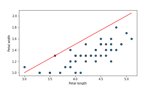
plot of chunk unnamed-chunk-65
## 0.5631599999999998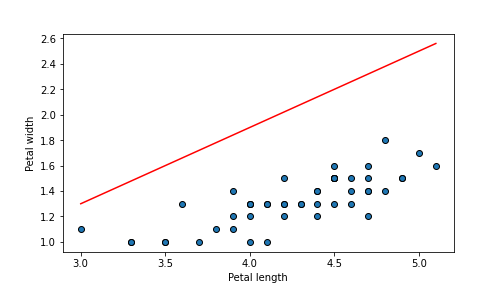
plot of chunk unnamed-chunk-65
## 0.030519999999999988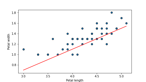
plot of chunk unnamed-chunk-65
## 0.01612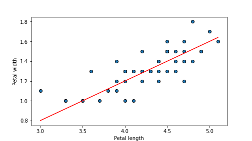
plot of chunk unnamed-chunk-65
A.7.1 Linear Regression in python: statsmodels.formula.api and sklearn
A.7.1.1 Solution: Explain virginica sepal width using linear regression with sklearn
from sklearn.linear_model import LinearRegression

iris = pd.read_csv("../data/iris.csv.bz2", sep="\t")
virginica = iris[iris.Species == "virginica"]
## extract explanatory variables as X
X = virginica[["Sepal.Length", "Petal.Width", "Petal.Length"]]
## call the dependent variable 'y' for consistency
y = virginica[["Sepal.Width"]]
m = LinearRegression()
_t = m.fit(X, y)
## compute R2
m.score(X, y)
## 0.39434712368959646A.7.1.2 Solution: Male wages as function of schooling and ethnicity
from sklearn.linear_model import LinearRegression

males = pd.read_csv("../data/males.csv.bz2", sep="\t")
## extract explanatory variables as X
X = males[["school", "ethn"]]
X.head(2)  # to see what it is
## school ethn
## 0 14 other
## 1 14 otherFor a check, let’s see what are the possible values of ethn:
## array(['other', 'black', 'hisp'], dtype=object)We have three different values. Hence we should have three coefficients as well–one for school and two for ethn as we drop one category as the reference.
Now we convert \(\mathsf{X}\) to dummies and fit the model
##       school  ethn_hisp  ethn_other
## 1246      12      False        True
## 436       15      False        True
## call the dependent variable 'y' for consistency
y = males[["wage"]]
m = LinearRegression()
_t = m.fit(X, y)Finally, check how many coefficients do we have:
## array([[0.07709427, 0.1471867 , 0.12256369]])Indeed, we have three coefficients. Compute \(R^2\):
## 0.06965044236285678A.7.2 Model Goodness
A.7.2.1 Solution: downward sloping, and well-aligned point clouds
Create downward trending point cloud: larger \(x\) must correspond to smaller \(y\), hence \(\beta_1\) should be negative. Choose \(\beta_1 = -1\):
n = 100
beta0, beta1 = 1, -1  # choose beta1 negative
x = np.random.normal(size=n)
eps = np.random.normal(size=n)
y = beta0 + beta1*x + eps
_t = plt.scatter(x, y, edgecolor="k")
_t = plt.xlabel("x")
_t = plt.ylabel("y")
_t = plt.show()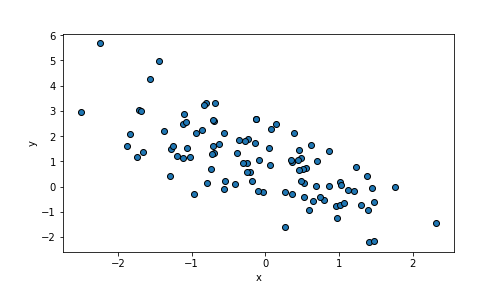
plot of chunk unnamed-chunk-72
scale defines the variation of the random values, the default value
is 1. As we add
\(\epsilon\) when computing \(y\), it describes how much the \(y\) values
are off from the perfect alignment:
n = 100
beta0, beta1 = 1, -1
x = np.random.normal(size=n)
eps = np.random.normal(scale=0.1, size=n)  # make eps small
y = beta0 + beta1*x + eps
_t = plt.scatter(x, y, edgecolor="k")
_t = plt.xlabel("x")
_t = plt.ylabel("y")
_t = plt.show()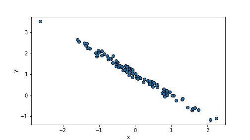
plot of chunk unnamed-chunk-73
A.7.2.2 Solution: Manually compute \(R^2\) for regression
import statsmodels.formula.api as smf
# find TSS
TSS = np.sum((versicolor.pw - np.mean(versicolor.pw))**2)
# find predicted values
m = smf.ols("pw ~ pl", data=versicolor).fit()
beta0, beta1 = m.params[0], m.params[1]
## <string>:1: FutureWarning: Series.__getitem__ treating keys as positions is deprecated. In a future version, integer keys will always be treated as labels (consistent with DataFrame behavior). To access a value by position, use `ser.iloc[pos]`pwhat = beta0 + beta1*versicolor.pl
# find ESS
ESS = np.sum((versicolor.pw - pwhat)**2)
R2 = 1 - ESS/TSS
R2## 0.6188466815001422A.7.2.3 Solution: Create a large and a small \(R^2\) value
Small variance (scale parameter) of \(\epsilon\) results in
well-aligned datapoints and hence high \(R^2\). E.g.
n = 100
beta0, beta1 = 1, -1  # choose beta1 negative
x = np.random.normal(size=n)
eps = np.random.normal(scale=0.05, size=n)
y = beta0 + beta1*x + eps
plt.scatter(x, y, edgecolor="k")
plt.xlabel("x")
plt.ylabel("y")
plt.show()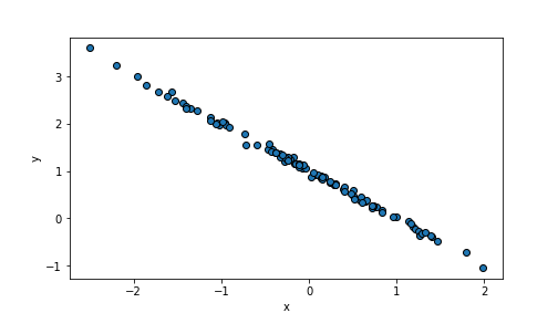
plot of chunk unnamed-chunk-75
randomDF = pd.DataFrame({"x":x, "y":y})
m = smf.ols("y ~ x", data=randomDF).fit()  # fit the model
m.rsquared
## 0.9977300775309055In contrary, a large variance of the error term makes points very weakly aligned with the regression line:
eps = np.random.normal(scale=5, size=n)
y = beta0 + beta1*x + eps
plt.scatter(x, y, edgecolor="k")
plt.xlabel("x")
plt.ylabel("y")
plt.show()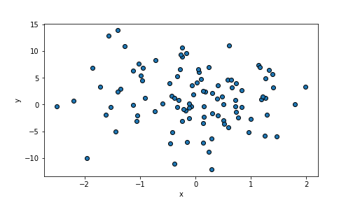
plot of chunk unnamed-chunk-76
randomDF = pd.DataFrame({"x":x, "y":y})
m = smf.ols("y ~ x", data=randomDF).fit()  # fit the model
m.rsquared
## 0.12166696652138498A.8 Logistic Regression
A.8.1 Logistic Regression in python: statsmodels.formula.api and sklearn
A.8.1.1 Solution: Predict treatment using all variables
First we load data, and convert all non-numeric variables to dummies.
##    treat  age  educ   ethn  married  re74  re75      re78   u74   u75
## 0   True   37    11  black     True   0.0   0.0   9930.05  True  True
## 1   True   30    12  black    False   0.0   0.0  24909.50  True  True
y = treatment.treat
## There are categoricals: convert these to dummies
X = pd.get_dummies(treatment.drop("treat", axis=1), drop_first=True)
## get a glimpse of X--does it look good?
X.sample(3)## age educ married ... u75 ethn_hispanic ethn_other
## 109 20 11 False ... False False False
## 781 35 9 True ... False False False
## 740 36 11 True ... False False False
##
## [3 rows x 10 columns]The design matrix looks reasonable. Note that logical values are kept as they are and not transformed to dummies–logical values are essentially dummies already. Now fit the model:
## /usr/lib/python3/dist-packages/sklearn/linear_model/_logistic.py:469: ConvergenceWarning: lbfgs failed to converge (status=1):
## STOP: TOTAL NO. of ITERATIONS REACHED LIMIT.
##
## Increase the number of iterations (max_iter) or scale the data as shown in:
##     https://scikit-learn.org/stable/modules/preprocessing.html
## Please also refer to the documentation for alternative solver options:
##     https://scikit-learn.org/stable/modules/linear_model.html#logistic-regression
## n_iter_i = _check_optimize_result(## 0.9652336448598131Indeed, score is now better than 93%.
A.9 Predictions and Model Goodness
A.9.1 Predicting using linear regression
A.9.1.1 Solution: manually predict distance to galaxies using modern data
hubble = pd.read_csv("../data/hubble.csv", sep="\t")

## fit with modern values
m = smf.ols("Rmodern ~ vModern", data=hubble).fit()
## assign estimated parameter values
beta0, beta1 = m.params

v7331 = hubble.vModern.iloc[17]
v7331  # velocity
## 816.0## 12.205922925181298## array([ 8.20010195, 14.53842628, 27.21507493])A.9.1.2 Solution: predict petal width
from sklearn.linear_model import LinearRegression

iris = pd.read_csv("../data/iris.csv.bz2", sep="\t")
versicolor = iris[iris.Species == "versicolor"]
y = versicolor[["Petal.Width"]]
X = versicolor[["Sepal.Length", "Sepal.Width"]]
# note: length first, width second
## get a glimpse of X--does it look good?
X.sample(3)
## Sepal.Length Sepal.Width
## 84 5.4 3.0
## 59 5.2 2.7
## 92 5.8 2.6## initialize and fit the model
m = LinearRegression()
_t = m.fit(X, y)
## predict
yhat = m.predict(X)
rmse = np.sqrt(np.mean((y - yhat)**2))
rmse## 0.1391612068531179RMSE is rather small, 0.1391612cm. This is because the range of petal width is small, only 0.8 cm.
In order to predict the flower of given size, we can create a matrix with the requested numbers:
## /usr/lib/python3/dist-packages/sklearn/base.py:493: UserWarning: X does not have valid feature names, but LinearRegression was fitted with feature names
##   warnings.warn(
## array([[0.97560275]])
A.9.1.3 Solution: predict hispanic male wage in service sector
As the first step we should load data check how is industry coded:
## array(['Business_and_Repair_Service', 'Personal_Service', 'Trade',
##        'Construction', 'Manufacturing', 'Transportation',
##        'Professional_and_Related Service', 'Finance', 'Entertainment',
##        'Public_Administration', 'Agricultural', 'Mining'], dtype=object)
We see that finance is coded just as “Finance”. Now we can follow the example in Section :
As second step we can fit the linear regression. We call the original
data matrix with categorical Xc in order to distinguish it from the
final design matrix X below:
from sklearn.linear_model import LinearRegression

## Extract relevant variables in original categorical form
## we need it below
Xc = males[["school", "ethn", "industry"]]
y = males.wage
X = pd.get_dummies(Xc, drop_first=True)
m = LinearRegression()
_t = m.fit(X, y)
Now m is a fitted model that we can use for prediction. Next, we
design the data frame for prediction using the categories and attach
it on top of the original categorical data matrix Xc:
## design prediction
newDf = pd.DataFrame({"school":16, "ethn":"hisp",
                      "industry":"Finance"},
                     index=["c1"])
## merge new on top of original
newDf = pd.concat((newDf, Xc), axis=0, sort=False)
## Does it look good?
newDf.head(3)
## school ethn industry
## c1 16 hisp Finance
## 0 14 other Business_and_Repair_Service
## 1 14 other Personal_Service## create dummies of everything
allX = pd.get_dummies(newDf, drop_first=True)
## do dummies look reasonable?
allX.head(3)## school ethn_hisp ... industry_Trade industry_Transportation
## c1 16 True ... False False
## 0 14 False ... False False
## 1 14 False ... False False
##
## [3 rows x 14 columns]Finally, we extract the relevant cases from the extended design matrix and predict:
##     school  ethn_hisp  ...  industry_Trade  industry_Transportation
## c1      16       True  ...           False                    False
##
## [1 rows x 14 columns]## array([2.16154055])Predicted hourly salary is $2.16.
A.9.2 Predicting with Logistic Regression
A.9.2.1 Solution: Predict Titanic survival for two persons using statsmodels
Load data and fit the model:
titanic = pd.read_csv("../data/titanic.csv.bz2")

m = smf.logit("survived ~ sex + C(pclass)", data=titanic).fit()
## Optimization terminated successfully.
## Current function value: 0.480222
## Iterations 6Next, create data for the desired cases. A simple way is to use dict of lists. We put the man at the first position and the woman at the second position:
## create new data (a dict)
## man in 1st class, woman in 3rd class
newx = {"sex":["male", "female"], "pclass":[1, 3]}
Now we can predict using these data:
## 0    0.399903
## 1    0.595320
## dtype: float64## 0 False
## 1 True
## dtype: boolAs the results indicate, a 1st class man has approximately 40% percent chance to survive, while a 3rd class woman has 60%. Hence we predict that the man died while the woman survived.
A.9.2.2 Solution: Test different thresholds with statsmodels
Load data and fit the model:
titanic = pd.read_csv("../data/titanic.csv.bz2")

m = smf.logit("survived ~ sex + C(pclass)", data=titanic).fit()
## Optimization terminated successfully.
## Current function value: 0.480222
## Iterations 6Predict the probabilities:
Now try a few different thresholds:
## 0.7799847211611918## 0.7203972498090145## 0.7364400305576776So far, 0.5 seems to be the best option.
For the plot, we can just create an array of thresholds and compute accuracy for each of these in a loop:
thresholds = np.linspace(0, 1, 100)
accuracies = np.empty(100)
for i in range(100):
    yhat = phat > thresholds[i]
    accuracies[i] = np.mean(yhat == titanic.survived)
_t = plt.plot(thresholds, accuracies)
_t = plt.xlabel("Threshold")
_t = plt.ylabel("Accuracy")
_t = plt.show()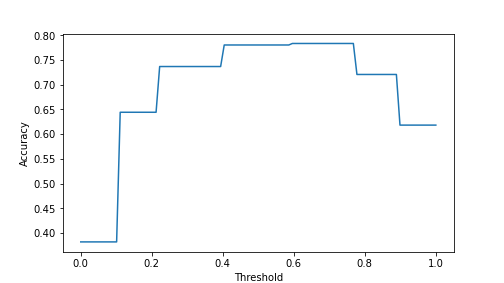
plot of chunk unnamed-chunk-92
The plot shows that the best accuracy is achieved at threshold value 0.6..0.7. This is, obviously, data dependent.
A.9.2.3 Solution: Row of four zeros
The object is a pandas data frame, and hence the first column–the first zero–is its index. This means we are using the first row of data.
The second column corresponds to dummy sex_male. Hence the person in
the first row is a female.
The 3rd and 4th columns are dummies, describing the passenger class. Hence together they indicate that the passenger was traveling in the 1st class.
To conclude: the zeros show that the passenger in the first line of data was a woman who was traveling in first class.
A.9.2.4 Solution: Predict treatment status using all variables
First load data and convert all non-numeric variables to dummies:
treatment = pd.read_csv("../data/treatment.csv.bz2", sep="\t")
y = treatment.treat
## drop outcome (treat) and convert all categoricals
## to dummmies
X = pd.get_dummies(treatment.drop("treat", axis=1), drop_first=True)
## get a glimpse of X--does it look good?
X.sample(3)
## age educ married ... u75 ethn_hispanic ethn_other
## 2523 48 8 True ... False False True
## 1972 32 12 True ... False False True
## 282 27 12 True ... False False False
##
## [3 rows x 10 columns]The design matrix looks reasonable, in particular we can see that the logical married is still logical, but ethn with three categories is converted to two dummies (ethn_hispanic and ethnc_other). Now fit the model:
## /usr/lib/python3/dist-packages/sklearn/linear_model/_logistic.py:469: ConvergenceWarning: lbfgs failed to converge (status=1):
## STOP: TOTAL NO. of ITERATIONS REACHED LIMIT.
##
## Increase the number of iterations (max_iter) or scale the data as shown in:
##     https://scikit-learn.org/stable/modules/preprocessing.html
## Please also refer to the documentation for alternative solver options:
##     https://scikit-learn.org/stable/modules/linear_model.html#logistic-regression
##   n_iter_i = _check_optimize_result(
Now we can extract the desired cases and predict values for those only:
newx = X.loc[[0, 9, 99]]  # extract desired rows
m.predict_proba(newx)[:,1]  # note: only output treatment probability
## array([0.36786129, 0.92517117, 0.63551329])As the probabilities suggest, the first case is predicted not to participate, and two latter cases are predicted to participate.
A.9.3 Confusion Matrix–Based Model Goodness Measures
A.9.3.1 Solution: Titanic Suvival Confusion Matrix with Child Variable
We can create child with a simple logical operation:
Note that we do not have to include child in the data frame, a variable in the working environment will do. Now we model and predict
## Optimization terminated successfully.
##          Current function value: 0.471565
## Iterations 6The confusion matrices, computed in two ways:
## col_0     False  True
## survived
## 0           682    127
## 1 156 344## array([[682, 127],
## [156, 344]])Indeed, both ways to get the matrix yield the same result.
And finally we extract true negatives:
## 682## 682This is the same number as in the original model in Section 12.3.2. But now we have slightly larger number of true positives.
A.9.3.2 Solution: Titanic Survival with Naive Model
We can create a naive model with formula "survived ~ 1" but let’s do
it manually here. We just predict everyone to the class that is more
common:
## survived
## 0    809
## 1    500
## Name: count, dtype: int64
As one can see, surival 0 is the more common value, hence we predict
everyone died:
In order to better understand the results, let’s also output the confusion matrix:
## col_0       0
## survived
## 0         809
## 1         500
As one can see, pd.crosstab only outputs a single column here, as we
do not predict anyone to survive. Essentially the survivor column is
all zeros but pd.crosstab does not show this (confusion_matrix
will show this column).
We can compute the goodness values using the sklearn.metrics:
from sklearn.metrics import accuracy_score, precision_score, recall_score, f1_score
accuracy_score(titanic.survived, yhat)
## 0.6180290297937356## /usr/lib/python3/dist-packages/sklearn/metrics/_classification.py:1509: UndefinedMetricWarning: Precision is ill-defined and being set to 0.0 due to no predicted samples. Use `zero_division` parameter to control this behavior.
## _warn_prf(average, modifier, f"{metric.capitalize()} is", len(result))
## 0.0## 0.0## 0.0The results give us two errors: as we do not predict any survivors, we cannot compute precision as 0 out of 0 predicted survivors are correct. As \(F\)-score is (partly) based on precision, we cannot compute that either. Additionally, \(R=0\) as we do not capture any survivors.
A.10 Trees and Forests
A.10.1 Regression Trees
A.10.1.1 Solution:
First load and prepare data:
from sklearn.tree import DecisionTreeRegressor

boston = pd.read_csv("../data/boston.csv.bz2", sep="\t")
## define outcome (medv) and design matrix (X)
y = boston.medv
X = boston[["rm", "age"]]
Now define and fit the model:
Compute \(R^2\) on training data:
## 0.6091083830815363This is a slight improvement, the original \(R^2\), using only rm, was 0.58. Hence the trees found it useful to include age in the decision-making. As the depth-2 tree is a very simple model, we are not really afraid of overfitting here.

Depth-2 Boston regression tree using both rm and age.
Here is the tree as seen by graphviz.
Indeed, now the tree considers age in the left node, with newer neighborhoods being somewhat more expensive.
Include all features:
## 0.695574477973027\(R^2\) improved noticeably. This hints that the tree was able to pick at least one other feature that was better to describe the price than rm and age.

Depth-2 Boston regression tree using all features.
Here is the tree when using all available features. rm is still the first feature to split data, but the other one is not lstat, the percentage of lower-status population.
A.11 Neural-networks
A.11.1 Using scalars for coding perceptrons
A.11.1.1 Vectors instead of scalars
Yes, it will work. There are only three operations involved: *, +
and >. All these work if you have a vector on one side and a scalar
on the other side.
Here’s the proof:
x1 = np.array([0, 0, 1, 1])
x2 = np.array([0, 1, 0, 1])
w1, w2 = 1, 1
zbar = 1.5

## Compute
z = w1*x1 + w2*x2
y = (z > zbar) + 0  # convert to a number
y
## array([0, 0, 0, 1])A.12 Machine learning techniques
A.12.1 Gradient descent
A.12.1.1 Compute gradient of \(\exp(-\boldsymbol{x}\cdot\boldsymbol{x}')\)
- We can almost literally copy the function definition into python, just
remember that matrix product is
@:
- Compute at given values:
## array([[0.36787944]])## array([[0.36787944]])## array([[0.13533528]])- Gradient: in scalar form: \[\begin{equation*} \nabla f(x_{1}, x_{2}) = \begin{pmatrix} -2x_{1} e^{-(x_{1}^{2} + x_{2}^{2})}\\ -2x_{2} e^{-(x_{1}^{2} + x_{2}^{2})} \end{pmatrix} = \begin{pmatrix} -2x_{1} f(x_{1}, x_{2})\\ -2x_{2} f(x_{1}, x_{2}) \end{pmatrix}. \end{equation*}\] Transforming it back in vector form: \(\nabla f(\boldsymbol{x}) = -2 \boldsymbol{x} f(\boldsymbol{x})\)
- This is a straightforward translation from math to python:
- Compute the gradients:
## array([[ 0.        ],
## [-0.73575888]])## array([[-0.73575888],
## [ 0. ]])## array([[-0.27067057],
## [-0.27067057]])- for 4-D case: the function and gradient will work perfectly. This is because because both are implemnted with vector operations only (no element-wise operations), and the inner product \(-\boldsymbol{x} \cdot \boldsymbol{x}'\) works for any dimension. Try it:
## array([[ 0.00000000e+00],
##        [-1.66305744e-06],
##        [-3.32611488e-06],
##        [-4.98917231e-06]])
A.13 Natural Language Processing
A.13.1 Categorize text
A.13.1.1 Dimension of DTM
Xhas 4 rows because our training data contains four documents.- It has 118 columns because that is the number of unique tokens in all training documents.
A.13.1.2 Detect the author of the poems with TF-IDF
We basically just swap CountVectorizer out for TfidfVectorizer.
Everything else will remain the same:
from sklearn.feature_extraction.text import TfidfVectorizer
vrizer = TfidfVectorizer()
X = vrizer.fit_transform([rudaki1, rudaki2, phu1, phu2])
newX = vrizer.transform([newdoc])

from sklearn.neighbors import NearestNeighbors
m = NearestNeighbors(n_neighbors=1, metric="cosine")
_t = m.fit(X)
d = m.kneighbors(newX, n_neighbors=4)
d
## (array([[0.44494572, 0.64788098, 0.78482153, 0.89982691]]), array([[2, 3, 1, 0]]))The closest document based on cosine distance is document 2 at distance 0.445.
To be more precise, they are not the riches, but those with the largest income in this data.↩︎