Chapter 10 Linear Regression

We assume you have loaded the following packages:

import numpy as np
import pandas as pd
import matplotlib.pyplot as plt

Below we load more as we introduce more.

10.1 Solving Linear Regression Tasks Manually

10.1.1 The task

In case of simple regression, the task is to find parameters \(\beta_0\) and \(\beta_1\) such that the mean squared error (MSE) is minimized wher MSE is defined as \[\begin{equation} MSE = \frac{1}{n}\sum_i (y_i - \hat y(x_i))^2 \end{equation}\] where the predicted value \[\begin{equation} \hat y(x_i) = \beta_0 + \beta_1\cdot x_i. \end{equation}\] Here \(n\) is the number of observations, \(x\) is our exogenous variable, and \(y\) is the outcome variable, and \(i\) indexes the observations. Normally we want to use software to perform this optimization (even more, this problem can be solved analytically) but it is instructive to attempt to solve the problem by hand.

Let us experiment with iris data and estimate the relationship between petal width and length of versicolor flowers. This is one of the most popular statistics and machine learning dataset, the version we use here originates from R datasets. You can download it from the Bitbucket repo of these notes. The dataset itself contains three species, and as their leaves may have different relationship, we filter out only one of those, versicolor. Also, as the variable names in this file are not suitable for modeling below, we rename variable called Petal.Length to plength, and Petal.Width to pwidth.

First we load the data, and thereafter filter with rename chained at the end of the filtering operation:

iris = pd.read_csv("../data/iris.csv.bz2", sep="\t")
# select only versicolor species,
# make variable names easier to handle
versicolor = iris[iris.Species == "versicolor"].rename(
    columns={"Petal.Length": "plength", "Petal.Width":"pwidth"})
# check if data looks reasonable
versicolor.head(3)

##     Sepal.Length  Sepal.Width  plength  pwidth     Species
## 50           7.0          3.2      4.7     1.4  versicolor
## 51           6.4          3.2      4.5     1.5  versicolor
## 52           6.9          3.1      4.9     1.5  versicolor

plt.scatter(versicolor.plength, versicolor.pwidth, edgecolor="k")
plt.xlabel("Petal length (cm)")
plt.ylabel("Petal width (cm)")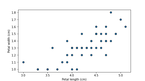

plot of chunk plotIris

The plot reveals that lengths and widths are positively correlated. This is to be expected, longer leaves are wider too.

10.1.2 Solve it manually

Denote petal length by \(l\) and petal width by \(w\). Solving the problem manually involves the following steps:

Pick suitable values for \(\beta_0\) and \(\beta_1\).
Compute the predicted petal width, \(\hat w_i = \beta_0 + \beta_1\cdot l_i\).
Computing the deviations \(e_i = w_i - \hat w_i\).
Compute MSE as \(MSE = \frac{1}{N} \sum_i e_i^2\).

Let us first write standalone code to perform these steps, and thereafter put all this into a function.

For a start, we can pick \(\beta_0 = 0\) and \(\beta_1 = 1\). This would amount to quadratic (or circular) leaves:

beta0, beta1 = 0, 1

Now we compute the predicted values. Remember, the petal length is called plength and petal widht is called pw in the versicolor dataframe:

hat_w = beta0 + beta1*versicolor.plength  # note: vectorized operators!
hat_w.head(3)  # this is a series!

## 50    4.7
## 51    4.5
## 52    4.9
## Name: plength, dtype: float64

The results are too wide–the true values are roughly 1.5, not 4.5. Apparently the choice of \(\beta_0\) and \(\beta_1\) was not a good one.

Compute deviations \(e_i\):

e = versicolor.pwidth - hat_w
e.head(3)

## 50   -3.3
## 51   -3.0
## 52   -3.4
## dtype: float64

Finally, compute MSE. Note that we can use the built-in np.mean to achieve this:

mse = np.mean(e**2)
mse

## 8.719800000000003

We get an \(MSE \approx 8.72\). This number in isolation does not tell much, but one can pick a different set of parameters \(\beta_0\) and \(\beta_1\), and compare the resulting MSE-s. This allows us to tell which choice is better.

10.1.3 Create a function to make it more compact

Now we can wrap these steps into a function to make the code more compact. The function might take two arguments, \(\beta_0\) and \(\beta_1\), so we can easily play with different values:

def mse(beta0, beta1):
    hat_w = beta0 + beta1*versicolor.plength  # note: vectorized operators!
    e = versicolor.pwidth - hat_w
    mse = np.mean(e**2)
    return mse

Now we can quickly try a few different parameter values to find out which combination works better:

mse(0, 1)  # this is what we did

## 8.719800000000003

mse(0, 0.5)  # this is better

## 0.6671999999999998

mse(-0.5, 0.5)  # even better!

## 0.11320000000000001

So out of these three attempts, the best parameter values are \(\beta_0 = -0.5\) and \(\beta_1 = 0.5\).

10.1.4 Visualize the Regression Line

So far we just computed \(MSE\) but we can do even better–we can also visualize the regression line. Matplotlib does not have a ready-made function to plot a regression line but it is easy to do by hand. We just create a number of sepal length values in a suitable range, predict the corresponding widths, and plot the results.

beta0, beta1 = -0.5, 0.5
# start by plotting the data
plt.scatter(versicolor.plength, versicolor.pwidth, edgecolor="k")
# create 11 evenly spaced lengths between the smallest and largest
# value in the data
length = np.linspace(versicolor.plength.min(), versicolor.plength.max(), 11)
# predict width
hatw = beta0 + beta1*length
plt.plot(length, hatw, c='r')
plt.xlabel("Petal length")
plt.ylabel("Petal width")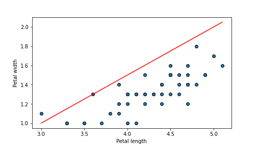

plot of chunk regressionLine

Despite the impressive \(MSE\) value, the figure shows that our line does not actually align well with data. We might continue trying different values to find an even better one.

Exercise 10.1 Write a function that takes \(\beta_0\) and \(\beta_1\) as arguments and a) computes \(MSE\) and b) plot the regression line. Experiment with the parameter values and find a combination that makes the line align well with the data points.

See the solution

10.2 Linear Regression in python: `statsmodels.formula.api` and `sklearn`

We discuss two popular libraries for doing linear regression in python. The first one, statsmodels.formula.api is useful if we want to interpret the model coefficients, explore \(t\)-values, and assess the overall model goodness. It is based on R-style formulas, and it provides well-designed summary tables. The other, sklearn, is more suitable for predictive modeling. Instead of formula it expects the design matrix, and it does not provide nicely formatted summary tables. However, it can be easily swapped with other predictive models in sklearn module.

10.2.1 Statsmodels and its formula API

We import the statsmodels formula API functionality as

import statsmodels.formula.api as smf

## /usr/lib/python3/dist-packages/scipy/__init__.py:146: UserWarning: A NumPy version >=1.17.3 and <1.25.0 is required for this version of SciPy (detected version 1.26.1
##   warnings.warn(f"A NumPy version >={np_minversion} and <{np_maxversion}"

It provides a number of statistical models, include ols, ordinary least squares, i.e. linear regression. The basic syntax of ols is

smf.ols(formula, data)

The formula is an R-style formula, such as "y ~ x1 + x2" and data is a data frame that contains the variables. For instance, the versicolor petal regression can be done as

m = smf.ols("pwidth ~ plength", data=versicolor)

This line just sets up the linear regression model but does not actually evaluate it, in order to get an answer, one has to add .fit():

m = smf.ols("pwidth ~ plength", data=versicolor).fit()

This results in evaluated model object m that provides several useful methods, in particular .params for parameter estimates, and .summary() for a summary table:

m.params

## Intercept   -0.084288
## plength      0.331054
## dtype: float64

m.summary()

OLS Regression Results
Dep. Variable:	pwidth	R-squared:	0.619
Model:	OLS	Adj. R-squared:	0.611
Method:	Least Squares	F-statistic:	77.93
Date:	Tue, 17 Sep 2024	Prob (F-statistic):	1.27e-11
Time:	19:52:49	Log-Likelihood:	34.709
No. Observations:	50	AIC:	-65.42
Df Residuals:	48	BIC:	-61.59
Df Model:	1
Covariance Type:	nonrobust

	coef	std err	t	P>\|t\|	[0.025	0.975]
Intercept	-0.0843	0.161	-0.525	0.602	-0.407	0.239
plength	0.3311	0.038	8.828	0.000	0.256	0.406

Omnibus:	0.204	Durbin-Watson:	2.412
Prob(Omnibus):	0.903	Jarque-Bera (JB):	0.002
Skew:	-0.012	Prob(JB):	0.999
Kurtosis:	3.017	Cond. No.	41.6

Notes:
[1] Standard Errors assume that the covariance matrix of the errors is correctly specified.

10.2.1.1 R-style formulas

The ability to enter formulas directly into the model is one of the strong sides of statsmodels.formula. This makes it easy to directly specify the dependent and independent variables given we have a data frame, there is no need to create an explicit design matrix (like in sklearn). These formulas originate from R where they are used in a similar fashion, that’s why they are called “R-style” formulas.

10.2.1.1.1 Specifying dependent and independent variables

The central part of the model formula is dependent - tilde - independent specification. We can write "y ~ x" and this will be understood as a linear regression model \[\begin{equation} y_i = \beta_0 + x_i \cdot \beta_1 + \epsilon_i. \end{equation}\] In particular what is before tilde ~ will be dependent variable (here \(y\)), and what is after tilde are independent variables (here just \(x\)). Unless explicitly requested not to, the model also include the intercept \(\beta_0\).

In case we have more independent variables, those can be added with plus sign, for instance "y ~ x1 + x2 + x3". This corresponds to the regression model \[\begin{equation} y_i = \beta_0 + x_{i1} \cdot \beta_1 + x_{i2} \cdot \beta_2 + x_{i3} \cdot \beta_3 + \epsilon_i. \end{equation}\] Hence the plus sign in the formula does not mean “add” but “include into the model”. So the formula should be read as "use \(y\) as the dependent variable, and include \(x_1\), \(x_2\) and \(x_3\) as explanatory variables.

For instance, if we want to estimate the median house value (medv) as a function of number of rooms (rm), percentage of lower-status population (lstat) and closeness to Charles river (chas), we can run the regression model like:

m = smf.ols("medv ~ rm + lstat + chas", data=boston).fit()

10.2.1.1.2 Categorical variables and interaction effects

Besides just specifying the variables, the formulas allow many more options. We use titanic data for the examples below.

First, note that if the variable is categorical (i.e. string) by design, it will be automatically converted to approriate dummies. For instance, sex is a categorical variable (with categories female and male) and hence it will be automatically converted into dummies. For instance, if we want to estimate a model \[\begin{equation} \text{survived}_i = \beta_0 + \text{male}_i \cdot \beta_1 + \epsilon_i, \end{equation}\] we can just insert string variable sex into the model:

titanic = pd.read_csv("../data/titanic.csv.bz2")
m = smf.ols("survived ~ sex", data=titanic).fit()
m.summary()

OLS Regression Results
Dep. Variable:	survived	R-squared:	0.280
Model:	OLS	Adj. R-squared:	0.279
Method:	Least Squares	F-statistic:	507.1
Date:	Tue, 17 Sep 2024	Prob (F-statistic):	3.78e-95
Time:	19:52:50	Log-Likelihood:	-697.97
No. Observations:	1309	AIC:	1400.
Df Residuals:	1307	BIC:	1410.
Df Model:	1
Covariance Type:	nonrobust

	coef	std err	t	P>\|t\|	[0.025	0.975]
Intercept	0.7275	0.019	38.049	0.000	0.690	0.765
sex[T.male]	-0.5365	0.024	-22.518	0.000	-0.583	-0.490

Omnibus:	37.339	Durbin-Watson:	1.611
Prob(Omnibus):	0.000	Jarque-Bera (JB):	39.798
Skew:	0.419	Prob(JB):	2.28e-09
Kurtosis:	2.834	Cond. No.	3.11

Notes:
[1] Standard Errors assume that the covariance matrix of the errors is correctly specified.

The line sex[T.male] shows the effect of male dummy with female being the reference group. This is because the categories will be ordered alphabetically, and the first (female) taken as the reference category.

But sometimes the categories are not strings but have numeric lables. For instance, male may be labeled as 1 and female as 2. Or, as is the case of titanic, we have numeric labels for passenger classes. Let us analyze the survival by passenger class using a model like \[\begin{equation} \text{survived}_i = \beta_0 + \text{class2}_i \cdot \beta_1 + \text{class3}_i \cdot \beta_2 + \epsilon_i, \end{equation}\] If we just specify the model as

smf.ols("survived ~ pclass", data=titanic)

pclass will be treated as a numeric variable, and the estimate should be interpreted as the effect per “one unit larger pclass”. This clearly does not make any sense. Instead, we have to tell statsmodels that pclass is a categorical variable by wrapping pclass into C function:

m = smf.ols("survived ~ C(pclass)", data=titanic).fit()
m.summary()

OLS Regression Results
Dep. Variable:	survived	R-squared:	0.098
Model:	OLS	Adj. R-squared:	0.096
Method:	Least Squares	F-statistic:	70.69
Date:	Tue, 17 Sep 2024	Prob (F-statistic):	7.10e-30
Time:	19:52:50	Log-Likelihood:	-845.26
No. Observations:	1309	AIC:	1697.
Df Residuals:	1306	BIC:	1712.
Df Model:	2
Covariance Type:	nonrobust

	coef	std err	t	P>\|t\|	[0.025	0.975]
Intercept	0.6192	0.026	24.084	0.000	0.569	0.670
C(pclass)[T.2]	-0.1896	0.038	-5.011	0.000	-0.264	-0.115
C(pclass)[T.3]	-0.3639	0.031	-11.732	0.000	-0.425	-0.303

Omnibus:	14135.138	Durbin-Watson:	1.846
Prob(Omnibus):	0.000	Jarque-Bera (JB):	142.320
Skew:	0.446	Prob(JB):	1.25e-31
Kurtosis:	1.653	Cond. No.	4.51

Notes:
[1] Standard Errors assume that the covariance matrix of the errors is correctly specified.

Now pclass will automatically be converted into dummies with 1 being the reference catogory. The lines C(pclass)[T.2] and C(pclass)[T.3] describe the effect of 2nd and 3rd class travel respectively (and reveal a sad story of lower survival chance for lower-class passengers).

We may also want to introduce gender and class interaction effects to test whether the survival rate depends on class, and whether this dependence differs for mean and women. This can be achieved with interaction effects in the form \(\text{male} \times \text{class}\), the full model would look like \[\begin{align*} \text{survived}_i &= \beta_0 + \text{class2}_i \cdot \beta_1 + \text{class3}_i \cdot \beta_2 + \\ & + \text{male}_i \cdot \beta_3 + \\ & + \text{class2}_i \cdot \text{male}_i \cdot \beta_4 + \text{class3}_i \cdot \text{male}_i \cdot \beta_5 + \epsilon_i. \end{align*}\] Interaction effects can be intered with asterisk *. For instance, x1 * x2 will include three variables: \(x_1\), \(x_2\), and \(x_1 \times x_2\). If any of the variables is categorical (either string or converted to categorical using C, the interaction effects will be inserted for all categories. Hence the Titanic class and sex example can be done as:

m = smf.ols("survived ~ C(pclass)*sex", data=titanic).fit()
m.summary()

OLS Regression Results
Dep. Variable:	survived	R-squared:	0.370
Model:	OLS	Adj. R-squared:	0.368
Method:	Least Squares	F-statistic:	153.2
Date:	Tue, 17 Sep 2024	Prob (F-statistic):	4.02e-128
Time:	19:52:50	Log-Likelihood:	-609.86
No. Observations:	1309	AIC:	1232.
Df Residuals:	1303	BIC:	1263.
Df Model:	5
Covariance Type:	nonrobust

	coef	std err	t	P>\|t\|	[0.025	0.975]
Intercept	0.9653	0.032	29.974	0.000	0.902	1.028
C(pclass)[T.2]	-0.0785	0.049	-1.587	0.113	-0.176	0.019
C(pclass)[T.3]	-0.4745	0.042	-11.414	0.000	-0.556	-0.393
sex[T.male]	-0.6245	0.043	-14.436	0.000	-0.709	-0.540
C(pclass)[T.2]:sex[T.male]	-0.1161	0.064	-1.801	0.072	-0.243	0.010
C(pclass)[T.3]:sex[T.male]	0.2859	0.054	5.340	0.000	0.181	0.391

Omnibus:	113.251	Durbin-Watson:	1.746
Prob(Omnibus):	0.000	Jarque-Bera (JB):	142.526
Skew:	0.805	Prob(JB):	1.12e-31
Kurtosis:	3.136	Cond. No.	13.3

Notes:
[1] Standard Errors assume that the covariance matrix of the errors is correctly specified.

As visible from the table, all the variables from the model above are included, and the all the pclass categories are taken into account. The lines containing colon, C(pclass)[T.2]:sex[T.male] and C(pclass)[T.3]:sex[T.male], are the interaction effects for male and the corresponding passenger class.

10.2.1.1.3 Transforming variables

## [1] 1000   10

One can perform certain computations directly in the model formula. In this example we use a random subset of diamonds data from R’s ggplot2 package. The dataset contains information on diamonds’ price (variable price), mass (carat), and other characteristics we do not discuss here. A few sample lines of the dataset are

diamonds.head()

##    carat        cut color clarity  depth  table  price     x     y     z
## 0   1.40      Ideal     G     VS2   62.1   55.0  10427  7.12  7.05  4.40
## 1   0.52       Good     D     SI2   63.7   55.0   1293  5.11  5.10  3.25
## 2   0.70  Very Good     F     VS2   60.9   61.0   2812  5.66  5.71  3.46
## 3   1.74    Premium     I     SI2   62.2   58.0   7858  7.65  7.61  4.75
## 4   0.30      Ideal     E    VVS2   62.3   54.1    779  4.28  4.34  2.69

We model the price as a function of mass. First we use a linear-linear regression model \[\begin{equation} \text{price}_i = \beta_0 + \text{carat}_i \cdot \beta_1 + \epsilon_i: \end{equation}\]

m = smf.ols("price ~ carat", data=diamonds).fit()
m.summary()

OLS Regression Results
Dep. Variable:	price	R-squared:	0.838
Model:	OLS	Adj. R-squared:	0.838
Method:	Least Squares	F-statistic:	5152.
Date:	Tue, 17 Sep 2024	Prob (F-statistic):	0.00
Time:	19:52:52	Log-Likelihood:	-8765.7
No. Observations:	1000	AIC:	1.754e+04
Df Residuals:	998	BIC:	1.755e+04
Df Model:	1
Covariance Type:	nonrobust

	coef	std err	t	P>\|t\|	[0.025	0.975]
Intercept	-2129.9155	96.843	-21.993	0.000	-2319.955	-1939.876
carat	7543.6403	105.102	71.774	0.000	7337.394	7749.887

Omnibus:	380.954	Durbin-Watson:	1.895
Prob(Omnibus):	0.000	Jarque-Bera (JB):	4043.711
Skew:	1.435	Prob(JB):	0.00
Kurtosis:	12.424	Cond. No.	3.69

Notes:
[1] Standard Errors assume that the covariance matrix of the errors is correctly specified.

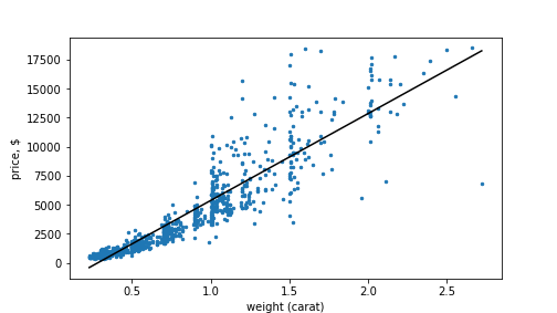
The results reveal that the price is closely related to the carat weight (coefficient value 7543.6 with a huge \(t\)-value). The model is also fairly good in terms of \(R^2 = 0.838\). But the plot below reveals that linear-linear model is not the best fit for the data:

plot of chunk diamondPlot

The figure suggest that the true price-weight curve is more convex, not the fact that the low-weight diamonds’ (ct < 0.5) price is consistently underpredicted, while those in range 0.5-1 are overpredicted. We may try log-log transformation instead. We may use functions directly to transform variables, in this case we can use np.log for log transform and write np.log(price) instead of price: \[\begin{equation} \log\text{price}_i = \beta_0 + \log\text{carat}_i \cdot \beta_1 + \epsilon_i: \end{equation}\]

m = smf.ols("np.log(price) ~ np.log(carat)", data=diamonds).fit()
m.summary()

OLS Regression Results
Dep. Variable:	np.log(price)	R-squared:	0.928
Model:	OLS	Adj. R-squared:	0.928
Method:	Least Squares	F-statistic:	1.284e+04
Date:	Tue, 17 Sep 2024	Prob (F-statistic):	0.00
Time:	19:52:53	Log-Likelihood:	-115.55
No. Observations:	1000	AIC:	235.1
Df Residuals:	998	BIC:	244.9
Df Model:	1
Covariance Type:	nonrobust

	coef	std err	t	P>\|t\|	[0.025	0.975]
Intercept	8.4414	0.010	810.896	0.000	8.421	8.462
np.log(carat)	1.6729	0.015	113.332	0.000	1.644	1.702

Omnibus:	16.775	Durbin-Watson:	1.940
Prob(Omnibus):	0.000	Jarque-Bera (JB):	26.702
Skew:	0.119	Prob(JB):	1.59e-06
Kurtosis:	3.764	Cond. No.	2.09

Notes:
[1] Standard Errors assume that the covariance matrix of the errors is correctly specified.

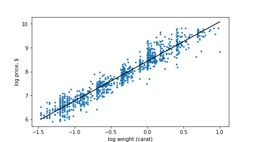
This model looks better as suggested by both \(R^2 = 0.928\) and the \(t\)-value. And here is the corresponding plot:

plot of chunk diamonds-log-log

Now the trend line looks perfectly straight and the linear model fits very well.

10.2.2 Scikit-learn and `LinearRegression`

Another very popular python library for linear regression is scikit-learn (usually abbreviated as sklearn). While statsmodels is mostly geared toward inference and provides nice summary tables with coefficients, \(t\) statistics and \(R^2\); sklearn is designed for predictive modeling. It does not provide similar output tables, and it does not have formula API. Instead, one has to create the design matrix manually, and use this when fitting the model. This may be somewhat complex if one needs some feature engineering, such as creating dummies. As an advantage though, it contains a large number of other predictive models with similar API, so swapping one model for another is very easy. It also contains other tools, such as cross-validation, that are commonly used for predictive modeling. However, some of the methods are implemented slightly differently than the textbook cases in statsmodels, in particular sklearn-versions often contain regularization switched on by default. So the results may turn out to be slightly different than what one may expect based on other implementations.

Below, we demonstrate how to use sklearn’s LinearRegression, Section 11.2.2 below explains how to perform logistic regression.

10.2.2.1 Numeric variables only

Let us start with the example of estimating the petal width of versicolor flowers (see Section 10.1.1). Linear regression can be performed using LinearRegression function:

# we have to import the model..
from sklearn.linear_model import LinearRegression
# .. and create the model
m = LinearRegression()

The import call makes the LinearRegression function available. The second line of code constructs the linear regression object that we can fit afterwards. It is similar to statsmodels call m = smf.ols("y ~ x", data=df), i.e. setting up the model without fitting it. LinearRegression takes various parameters, but here we are usually happy with the defaults. In particular, we are happy with the dafault behavior of adding the intercept to the model automatically, so we do not have to add a constant column to \(\mathsf{X}\).

Next, we have to construct the design matrix. Here it is easy, as it just contains a single numeric variable. But it must be a matrix (or data frame), not a vector. The following code fill fail:

## create design matrix
X = versicolor.plength
# problem: X is a series, not matrix!
m = LinearRegression()
_ = m.fit(X, versicolor.pwidth)

## ValueError: Expected a 2-dimensional container but got <class 'pandas.core.series.Series'> instead. Pass a DataFrame containing a single row (i.e. single sample) or a single column (i.e. single feature) instead.

Let us now ensure that our design matrix is a matrix and not a vector. We can achieve this by adding additional brackets around pl (see Section 3.3.1 for more explanations):

# create design matrix
X = versicolor[["plength"]]
# now X is a data frame
m = LinearRegression().fit(X, versicolor.pwidth)

Note the similarities and differences between statsmodels and sklearn: in both cases you first set up the model (either with ols() or LinearRegression()) and thereafter fit it with .fit() method. However, in case of statsmodels you supply data to the ols() function, in case of sklearn you supply it to .fit() method. Also, sklearn requires you to supply the design matrix X and target y separately. statsmodels will create these objects itself from the formula.

Now m is a fitted model. We can query the parameters as

m.intercept_  # intercept

## -0.08428835489833664

m.coef_  # the estimated parameters, here just one

## array([0.3310536])

You can see that these numbers are exactly the same as in Section @ref(#linear-regression-statsmodels).

One can query a quick model goodness summary using .score method. In case of linear regression (and other regression models) it returns \(R^2\):

m.score(X, versicolor.pwidth)

## 0.6188466815001425

Again, we get exactly the same number as when using statsmodels above. Note that .score method expects two arguments: the design matrix X and target y, in this order. (It is the same order as for the .fit method.) Internally it predicts the values for every row of X, computes errors between predictions and y, and transforms this to \(R^2\). But by supplying X and y to the .score-method we can calculate \(R^2\) on different data–on validation data instead of training data (see Section 13 for more information).

But sklearn does not have a function to print a similar summary table as what .summary does in statsmodels. We cannot easily see standard errors, \(p\)-values or statistical significance. sklearn is designed for predictive modeling where such tables are of little value. In complex cases, for instance in image processing, we may want to include values of millions of pixels into the model and here individual specification of each pixel is clearly infeasible. We prefer to use the design matrix approach instead. In a similar fashion, we are not interested in interpreting values of millions of coefficients. sklearn is designed for exactly such tasks.

TBD: exercise with a single variable (Hubble)

Exercise 10.2 Take the iris data. Extract data for virginica (where Species = virginica) and run a regression: \[\begin{equation} \text{sepal width}_i = \beta_0 + \beta_1 \cdot \text{sepal length}_i + \beta_2 \cdot \text{petal width}_i + \beta_3 \cdot \text{petal length}_i + \epsilon_i. \end{equation}\] Compute \(R^2\).

See the solution

10.2.2.2 Categorical variables

As sklearn does not include a formula method, one cannot rely on it to convert categoricals to dummies. Instead, one has to make dummies manually. A good choice will be to use pd.get_dummies function. As an example, let’s use the males dataset and estimate a regression model \[\begin{equation} \log w_i = \beta_0 + \beta_1 \cdot \text{school}_i + \beta_2 \cdot \text{residence}_i + \epsilon_i. \end{equation}\] Here \(\log w\) is log hourly wage (in 1980-s, called wage in the dataset), school is years of schooling, and residence is the residence region (“rural_area”, “north_east”, “nothern_central” and “south”).

As the first step, we have to create the design matrix X by including all the relevant variables and converting categoricals to dummies:

males = pd.read_csv("../data/males.csv.bz2", sep="\t")\
    [["wage", "school", "residence"]]
# a look at the original data
males.sample(3)

##           wage  school        residence
## 3184  2.238261      14              NaN
## 306   1.680934      10  nothern_central
## 1186  1.680934      12            south

The simplest approach we can do is just to convert all the explanatory variables (here school and residence) with pd.get_dummies and let it sort out what is numeric and what is not. We also ask one category to be dropped as the reference category:

X = pd.get_dummies(males[["school", "residence"]],
                   # do not include 'wage' into X!
                   drop_first=True)
X.sample(3)

##       school  residence_nothern_central  residence_rural_area  residence_south
## 3138       6                          0                     0                0
## 1520      12                          0                     0                0
## 1810      12                          1                     0                0

One can see that school was preserved as a numeric column, but the four-category residence was transformed into three columns (with north_east dropped as the reference category).

For consistency, we also separate the outcome, \(\log w\), into a vector \(\mathbf{y}\):

y = males.wage

Now this is a ready-made numeric matrix we can use for fitting sklearn models. We also need the outcome variable, here just the log-income males.wage. Now we can fit the model as

m = LinearRegression()
_ = m.fit(X, y)

LinearRegression()

In a Jupyter environment, please rerun this cell to show the HTML representation or trust the notebook.
On GitHub, the HTML representation is unable to render, please try loading this page with nbviewer.org.

we assign the result of .fit to a temporary variable—it returns the fitted object and we do not want it to be printed here.

As no output is visible, we may manually examine the results:

m.coef_  # vector of parameters (but not intercept)

LinearRegression()

We can see that .coef_ is a vector of four values–one for each column of X, in the same order as in the columns. So .coef[0] tells us that those who have spent one year more at school earn 8% more, at least in average. We also see that income in all regions is smaller than in the reference region, North-East.

We can compute \(R^2\) using the .score method, there are no differences with the only numeric case in Section 10.2.2.1:

m.score(X, y)

LinearRegression()

Exercise 10.3 Take the males dataset and run a regression: \[\begin{equation} \log w_i = \beta_0 + \beta_1 \cdot \text{school}_i + \beta_2 \cdot \text{ethn}_i + \epsilon_i. \end{equation}\] where school is years of schooling, and ethn is race categories.

Ensure you have correct number of coefficients. Compute \(R^2\).

See the solution

10.3 Model Goodness

10.3.1 Create Random Data for Experiments

Random data is useful for learning or testing methods for various reasons as they allow to design exactly the features we are interested in trying our methods on, and when manually creating data, we will also know what exactly do we put in there and hence also what we ought to get out. If our results do not agree, something is wrong either in our code or our understanding of the method.

For linear regression we can create data exactly as specified by the linear regression model: \[\begin{equation} y_i = \beta_0 + \beta_1 \cdot x_i + \epsilon_i. \end{equation}\] Here \(x\) is our explanatory variable. We do not have to specify precisely how it looks like, but random normals are a good bet. \(\epsilon\) is the random disturbance term, a term necessary to knock the points off from the straight line to make the artificial data to resemble real data. This should be normal to ensure that the estimated standard errors are correct. We also have to choose the values for parameters \(\beta_0\) and \(\beta_1\), in this example we choose 1 and 2. Let us create a dataset with 100 observations:

n = 100

LinearRegression()

beta0, beta1 = 1, 2

LinearRegression()

x = np.random.normal(size=n)  # create random x

LinearRegression()

eps = np.random.normal(size=n)  # random disturbance term

LinearRegression()

y = beta0 + beta1*x + eps  # create y exactly as specified by linear regression definiton

LinearRegression()

# finally, keep this data in a dataframe for future
randomDF = pd.DataFrame({"x":x, "y":y})

LinearRegression()

Let’s plot the resulting \(x\) and \(y\):

_ = plt.scatter(x, y, edgecolor="k")
_ = plt.xlabel("x")
_ = plt.ylabel("y")
_ = plt.show()

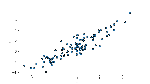
plot of chunk unnamed-chunk-34

We can see an upward-trending cloud of points.

Exercise 10.4

Modify the parameters \(\beta_0\) and \(\beta_1\) and create a downward trending point cloud
Modify the scale parameters of np.random.normal when creating \(\epsilon\) to create a point cloud that is very narrow (dots are almost perfectly lined up).

Show your data on a plot.

See the solution

10.3.2 Compute SSE, TSS, and \(R^2\) manually

In this example we use our random data frame we created above. As the first step, let’s compute TSS using the definition \[\begin{equation} \text{TSS} = \sum_{i=1}^{N} (y_{i} - \bar{y} )^{2}. \end{equation}\] This definition can be directly translated into computer code:

TSS = np.sum((y - np.mean(y))**2)
TSS

## 519.5528490036102

This is the total variation in the data (in \(y\)). How much will be left unexplained by linear regression? First we have to fit a linear regression model in order to be able to compute this:

m = smf.ols("y ~ x", data=randomDF).fit()  # fit the model
beta0 = m.params[0]  # assign the best solution coefficients to beta0, beta1
beta1 = m.params[1]

Now we can compute the predicted values in a fairly similar way as when we created random data. Just remember that we compute expected values as predictions, and hence we just ignore \(\epsilon\):

yhat = beta0 + beta1*x

Now we have both true values y and predicted values yhat. We can use the definition of SSE and compute deviations \(e\) and thereafter SSE:

e = y - yhat
SSE = np.sum(e**2)
SSE

## 99.95983754370855

Finally, we can also compute \(R^2\) from the definition:

R2 = 1 - SSE/TSS
R2

## 0.8076041008428501

We may want to compare our “home-made” \(R^2\) with the one provided by statsmodels rsquared attribute:

m.rsquared

## 0.8076041008428501

One can see that the the summary method provide a similar \(R^2\).

Exercise 10.5 Use the versicolor data to estimate a regression model \[\begin{equation} \text{Petal width}_{i} = \beta_{0} + \beta_{1} \cdot \text{Petal length} + \epsilon_{i}, \end{equation}\] the exact same model we used in Solving Linear Regression Tasks Manually. Compute \(R^2\) manually as we did above.

See the solution

Exercise 10.6 Modify your data generation procedure, in particular the scale parameter for \(\epsilon\) so that you get:

\(R^2 > 0.99\)
\(R^2 < 0.1\).

Show the corresponding data points on a plot.

See the solution

Chapter 10 Linear Regression

10.1 Solving Linear Regression Tasks Manually

10.1.1 The task

10.1.2 Solve it manually

10.1.3 Create a function to make it more compact

10.1.4 Visualize the Regression Line

10.2 Linear Regression in python: statsmodels.formula.api and sklearn

10.2.1 Statsmodels and its formula API

10.2.1.1 R-style formulas

10.2.1.1.1 Specifying dependent and independent variables

10.2.1.1.2 Categorical variables and interaction effects

10.2.1.1.3 Transforming variables

10.2.2 Scikit-learn and LinearRegression

10.2.2.1 Numeric variables only

10.2.2.2 Categorical variables

10.3 Model Goodness

10.3.1 Create Random Data for Experiments

10.3.2 Compute SSE, TSS, and \(R^2\) manually

10.2 Linear Regression in python: `statsmodels.formula.api` and `sklearn`

10.2.2 Scikit-learn and `LinearRegression`