Chapter 14 Machine Learning Workflow

We assume you have loaded the following packages:

import numpy as np
import pandas as pd
import matplotlib.pyplot as plt

Below we load more as we introduce more.

In this section we walk over a typical machine learning workflow using sklearn package. We assume you know what is overfitting and validation (see Section 13) and you are familiar with the basics of sklearn (see Section 10.2.2).

14.1 Model selection

This section demonstrates model selection–more specifically, how to choose between two logistic regression models that differ in terms of which features they contain. As a first step, you need to create the design matrix with eventual feature engineering, and as a second step, we compare the models using both validation set and cross-validation.

14.1.1 Prepare data

We use Titanic data (see Section 23.3):

titanic = pd.read_csv("../data/titanic.csv.bz2", sep = ",")
titanic.head(3)

##    pclass  survived  ... body                        home.dest
## 0       1         1  ...  NaN                     St Louis, MO
## 1       1         1  ...  NaN  Montreal, PQ / Chesterville, ON
## 2       1         0  ...  NaN  Montreal, PQ / Chesterville, ON
## 
## [3 rows x 14 columns]

We model the survival probability as a function of passenger class, sex and age. For simplicity, let’s use just a single variable child (True if age is less than 13), instead of age.

First, pick the subset of features, remove missings, and compute child:

titanic = titanic[["survived", "age", "pclass", "sex"]]
titanic = titanic.dropna(axis=0)
titanic["child"] = titanic.age < 13
titanic = titanic.drop("age", axis = 1)
titanic.shape

## (1046, 4)

Now we have dataset that looks like

titanic.sample(3)

##       survived  pclass     sex  child
## 1271         0       3    male  False
## 811          0       3  female  False
## 353          1       2  female  False

This will be all data for the first model. We need to create the design matrix and convert categoricals to dummies. I call the corresponding design matrix X1 because below we are using a different set of features and call that X2.

from sklearn.model_selection import train_test_split

y = titanic.survived
X = titanic.drop("survived", axis = 1)
X1 = pd.get_dummies(X, columns = ["sex", "pclass"])
X1.sample(3)

##       child  sex_female  sex_male  pclass_1  pclass_2  pclass_3
## 263   False        True     False      True     False     False
## 1266  False       False      True     False     False      True
## 353   False        True     False     False      True     False

As a second model, we will test if interaction effects between sex and pclass will improve the model. Conceptually, this means to test whether the gender effect differs between passenger classes. This may very well be the case. For this test, we need to make new columns that contain interaction effects. In this case, one could use the design matrix we already created, X1. However, I chose to do it on the original data instead:

titanic["male2"] = (titanic.sex == "male")*(titanic.pclass == 2)
titanic["male3"] = (titanic.sex == "male")*(titanic.pclass == 3)

Now we have two additional columns that capture males who were travelling in the 2nd and 3rd class respectively:

titanic.sample(3)

##      survived  pclass     sex  child  male2  male3
## 211         0       1    male  False  False  False
## 272         1       1  female  False  False  False
## 985         1       3    male  False  False   True

Finally, make dummies. We could include the new columns, male2 and male3, as the columns that need to be transformed into dummies. However, those are already logical values, and logical values are as good as dummies. So it is not needed in this case.

X = titanic.drop("survived", axis = 1)
X2 = pd.get_dummies(X, columns = ["sex", "pclass"])
X2.sample(3)

##       child  male2  male3  sex_female  sex_male  pclass_1  pclass_2  pclass_3
## 262   False  False  False       False      True      True     False     False
## 53    False  False  False       False      True      True     False     False
## 1130  False  False  False        True     False     False     False      True

14.1.2 Training-validation workflow

First we demonstate the workflow using training-validation approach. We split data into training and validation parts:

X1t, X1v, X2t, X2v, yt, yv = train_test_split(X1, X2, y, test_size = 0.2,
                                              random_state = 3)
X1t.shape

## (836, 6)

X2t.shape

## (836, 8)

I have chosen to do the same split for X2 and X3–in this way the results are better comparable and less dependent on the random split. (For consistency, I also specify the random state.)

Now we can test both models in terms of validation accuracy. For the first model:

from sklearn.linear_model import LogisticRegression

m = LogisticRegression()
_t = m.fit(X1t, yt)
m.score(X1v, yv)

## 0.8047619047619048

And for the second model:

m = LogisticRegression()
_t = m.fit(X2t, yt)
m.score(X2v, yv)

## 0.8095238095238095

In this case, the second model work better–but the difference is very very small. Personally, based on this analysis, I’d prefer the first model as that one is simpler.

14.1.3 Cross-validation

As a single training-validation split may be sensitive to the random split, it is advisable to use cross-validation (CV) instead. Below, I use 10-fold CV to compare the models.

There are multiple ways to perform cross-validation, perhaps the simples option is the function cross_val_score(). It needs you to specify the model (here m), the design matrix (here X1) and the outcome vector (here y). You can also specify the number of folds using the named argument cv (the default is 5):

from sklearn.model_selection import cross_val_score

cv = cross_val_score(m, X1, y, cv = 10)  # 10-fold
cv

## array([0.40952381, 0.86666667, 0.84761905, 0.82857143, 0.77142857,
##        0.8       , 0.80769231, 0.69230769, 0.64423077, 0.71153846])

np.mean(cv)

## np.float64(0.7379578754578755)

cross_val_score() returns a vector of the corresponding scores, normally we want to compare the averages between two models.

And for the second model we have

cv = cross_val_score(m, X2, y, cv = 10)
np.mean(cv)

## np.float64(0.7435439560439561)

You can see that the accuracy of the 2nd model is slightly better, by one percentage point.

cross_val_score() has many more arguments, the most important one, scoring, allows you to specify a different performance measure instead of accuracy.

TBD: exercise

14.2 Categorization: image recognition

Here we analyze MNIST digits. This is a dataset of handwritten digits, widely used for computer vision tasks. sklearn contains a low-resolution sample of this dataset:

from sklearn.datasets import load_digits
mnist = load_digits()
X = mnist.data
y = mnist.target

This loads the dataset and extracts the design matrix and labels y from there. We can take a look how does the data look with

X.shape

## (1797, 64)

y[:25]

## array([0, 1, 2, 3, 4, 5, 6, 7, 8, 9, 0, 1, 2, 3, 4, 5, 6, 7, 8, 9, 0, 1,
##        2, 3, 4])

X tells us that we have 1797 different digits, each of which contains 64 features. These features are pixels–the image consists of \(8\times8\) pixels, in the design matrix X the images are flattened into 64 consecutive pixels as features. A sample of data looks like

X[7:9]

## array([[ 0.,  0.,  7.,  8., 13., 16., 15.,  1.,  0.,  0.,  7.,  7.,  4.,
##         11., 12.,  0.,  0.,  0.,  0.,  0.,  8., 13.,  1.,  0.,  0.,  4.,
##          8.,  8., 15., 15.,  6.,  0.,  0.,  2., 11., 15., 15.,  4.,  0.,
##          0.,  0.,  0.,  0., 16.,  5.,  0.,  0.,  0.,  0.,  0.,  9., 15.,
##          1.,  0.,  0.,  0.,  0.,  0., 13.,  5.,  0.,  0.,  0.,  0.],
##        [ 0.,  0.,  9., 14.,  8.,  1.,  0.,  0.,  0.,  0., 12., 14., 14.,
##         12.,  0.,  0.,  0.,  0.,  9., 10.,  0., 15.,  4.,  0.,  0.,  0.,
##          3., 16., 12., 14.,  2.,  0.,  0.,  0.,  4., 16., 16.,  2.,  0.,
##          0.,  0.,  3., 16.,  8., 10., 13.,  2.,  0.,  0.,  1., 15.,  1.,
##          3., 16.,  8.,  0.,  0.,  0., 11., 16., 15., 11.,  1.,  0.]])

You can see many “0”-s (background) and numbers between “1” and “15”, denoting various intensity of the pen. We can easily plot these images, just we have to reshape those back into \(8\times8\) matrices. This is what is leads to

X[7].reshape((8,8))

## array([[ 0.,  0.,  7.,  8., 13., 16., 15.,  1.],
##        [ 0.,  0.,  7.,  7.,  4., 11., 12.,  0.],
##        [ 0.,  0.,  0.,  0.,  8., 13.,  1.,  0.],
##        [ 0.,  4.,  8.,  8., 15., 15.,  6.,  0.],
##        [ 0.,  2., 11., 15., 15.,  4.,  0.,  0.],
##        [ 0.,  0.,  0., 16.,  5.,  0.,  0.,  0.],
##        [ 0.,  0.,  9., 15.,  1.,  0.,  0.,  0.],
##        [ 0.,  0., 13.,  5.,  0.,  0.,  0.,  0.]])

If you look at the matrix closely, you can see that it depicts a number “7”. This is much easier to see if we plot the result:

plt.imshow(X[7].reshape((8,8)), cmap="gray_r")

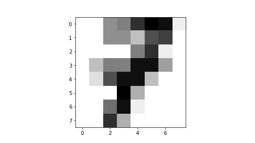
plot of chunk unnamed-chunk-19

This is a low-resolution image of number “7”. Here is a larger example of the first 30 digits:

for i in range(30):
    ax = plt.subplot(3, 10, i+1)
    _ = ax.imshow(X[i].reshape((8, 8)), cmap='gray_r')
    _ = ax.axis("off")
    _ = ax.set_title(f"A: {y[i]}")
_ = plt.show()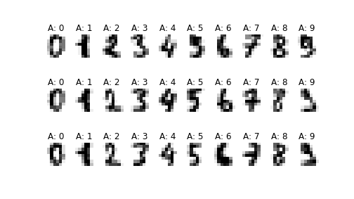

plot of chunk unnamed-chunk-20

As you can see, the numbers are of low quality and a bit hard to recognize for us. Computer will do it very well though–our brains are trained with high-quality images, not with low-quality images like here.

As a first step, let’s take an easy task and separate “0”-s and “1”-s. We’ll test a few different models in terms of how well do those perform. Extract all “0”-s and “1”-s:

## Find all 0,1 -s
i = np.isin(y, [0, 1])
Xd01 = X[i]
yd01 = y[i]

Next, we do training-validation split to validate our predictions:

Xt, Xv, yt, yv = train_test_split(Xd01, yd01)
Xt.shape, Xv.shape

## ((270, 64), (90, 64))

We can use logistic regression for this binary classification task, and after we fit the model, we compute accuracy:

from sklearn.linear_model import LogisticRegression

m = LogisticRegression()
_t = m.fit(Xt, yt)  # fit on 270 training cases
m.score(Xv, yv)  # validate on 90 validation cases

## 1.0

We got a perfect score–1.0. This means that the model is able to perfectly distinguish between these two digits. Indeed, these digits are in fact easy to distinguish, the pixel patterns look substantially different.

Let us try some more challenging tasks–to distinguish between “4”-s and “9”-s:

i = np.isin(y, [4, 9])
Xd01 = X[i]
yd01 = y[i]
Xt, Xv, yt, yv = train_test_split(Xd01, yd01)
_t = m.fit(Xt, yt)
m.score(Xv, yv)

## 1.0

The result is still ridiculously good with only a single wrong prediction as shown by the confusion matrix:

from sklearn.metrics import confusion_matrix
yhat = m.predict(Xv)
confusion_matrix(yv, yhat)

## array([[44,  0],
##        [ 0, 47]])

The mis-categorized image is

iw = yhat != yv  # which predictions are wrong
plt.imshow(Xv[iw].reshape((8, 8)), cmap='gray_r')

## ValueError: cannot reshape array of size 0 into shape (8,8)

plt.axis("off")

## (np.float64(0.0), np.float64(1.0), np.float64(0.0), np.float64(1.0))

plt.show()

plot of chunk unnamed-chunk-26

Indeed, even human eyes cannot tell what is the digit.

Logistic regression allows to use more than two categories–this is called multinomial logit. So instead of distinguishing between just two types of digits, we can categorize all 10 different categories:

from warnings import simplefilter
from sklearn.exceptions import ConvergenceWarning

simplefilter("ignore", category=ConvergenceWarning)

Xt, Xv, yt, yv = train_test_split(X, y)
m = LogisticRegression()
_t = m.fit(Xt, yt)
m.score(Xv, yv)

## 0.9755555555555555

The results are still very-very good although we got more than a single case wrong. The confusion matrix is

yhat = m.predict(Xv)
confusion_matrix(yv, yhat)

## array([[37,  0,  0,  0,  0,  0,  0,  0,  0,  0],
##        [ 0, 50,  0,  0,  1,  0,  0,  0,  0,  0],
##        [ 0,  0, 41,  0,  0,  0,  0,  0,  0,  0],
##        [ 0,  0,  0, 46,  0,  0,  0,  0,  0,  1],
##        [ 0,  1,  0,  0, 38,  0,  0,  0,  1,  0],
##        [ 0,  0,  0,  0,  0, 46,  0,  0,  0,  0],
##        [ 0,  0,  0,  0,  0,  0, 43,  0,  0,  0],
##        [ 0,  0,  0,  0,  0,  0,  0, 47,  1,  0],
##        [ 0,  3,  0,  0,  0,  1,  0,  0, 43,  0],
##        [ 0,  1,  0,  0,  0,  0,  0,  0,  1, 48]])

We can see that by far the most cases are on the main diagonal–the model gets most of the cases right. The most problematic cases are mispredicting “8” as “1”.

14.3 Training-validation-testing approach

We start by separating testing, or hold-out data:

Xw, Xh, yw, yh = train_test_split(X, y)
Xw.shape

## (1347, 64)

Now we do not touch the hold-out data until the very end. Instead, we split the work-data into training and validation parts:

Xt, Xv, yt, yv = train_test_split(Xw, yw)
Xt.shape

## (1010, 64)

Now we can test different models on training-validation data:

mLogistic = LogisticRegression(C=1e9)
mLogistic.fit(Xt, yt)

## LogisticRegression(C=1000000000.0)

mLogistic.score(Xv, yv)

## 0.9584569732937686

The beauty of sklearn is that is easy to try different models. Let’s try a single nearest-neighbor classifier:

from sklearn.neighbors import KNeighborsClassifier

m1NN = KNeighborsClassifier(1)
_t = m1NN.fit(Xt, yt)
m1NN.score(Xv, yv)

## 0.9910979228486647

This one achieved very good score on validation data. What about 5-nearest neighbors?

from sklearn.neighbors import KNeighborsClassifier

m5NN = KNeighborsClassifier(5)
_t = m5NN.fit(Xt, yt)
m5NN.score(Xv, yv)

## 0.9821958456973294

The accuracy is almost as good as in single-nearest-neighbor case. We can also try decision trees:

from sklearn.tree import DecisionTreeClassifier

mTree = DecisionTreeClassifier()
_t = mTree.fit(Xt, yt)
mTree.score(Xv, yv)

## 0.8664688427299704

Trees were clearly inferior here.

Instead of training-validation split, we can use cross-validation:

from sklearn.model_selection import cross_val_score

cross_val_score(mLogistic, Xw, yw, cv=5).mean()

## np.float64(0.9539749414842351)

cross_val_score(m1NN, Xw, yw, cv=5).mean()

## np.float64(0.989607600165221)

cross_val_score(m5NN, Xw, yw, cv=5).mean()

## np.float64(0.9829244114002478)

cross_val_score(mTree, Xw, yw, cv=5).mean()

## np.float64(0.8456120060581027)

Cross-validation basically replicated training-validation split results and the best model again appears to be 1-NN. But the lead in front of 5-NN is just tiny. But we can pick 1-NN as our preferred model.

Fianlly, the hold-out data gives us the final performance measure:

m1NN.score(Xh, yh)

## 0.9733333333333334

Now we have computed the final model accuracy, we should not change the model any more.