Chapter 11 Doing statistics with R

11.1 Random numbers

R has a very handy built-in random number functionality. It covers a number of common distributions, and allows to generate random numbers and calculate probability density (or mass), cumulative distribution, and distribution quantiles. All these functions, except sample(), use a standard interface.

11.1.1 Sampling elements: sample()

sample() samples elements from a vector. Its basic usage is sample(vector, n) that pulls out \(n\) random elements from the vector. For instance,

sample(1:10, 3)

## [1] 5 6 3

This takes three random elements out of the vector 1:10, i.e. out of numbers 1 to 10. By default, it extracts the elements without replacement, i.e. if number 5 is already taken, you cannot get that number again. If this is not what you wish, you can specify replace = TRUE to choose elements with replacement:

sample(c("A", "B"), 10, replace = TRUE)

##  [1] "B" "A" "A" "B" "B" "A" "B" "B" "A" "B"

This selects either “A” or “B” randomly for 10 times. This is obvioulsy impossible unless with select with replacement.

There is a handy shortcut to select numbers 1, 2, …, K: sample(K, n). So in order to emulate rolling a die you can write

sample(6, 1)  # one number between 1 and 6

## [1] 5

Exercise 11.1 You want to simulate rolling 5 dice. You write

sample(6, 5)

Is this correct?

The solution

One can also ask sample() to do non-uniform sampling. For instance

sample(c("A", "B"), 10, replace = TRUE,
       prob = c(3, 7))

##  [1] "B" "B" "A" "B" "B" "A" "B" "B" "B" "B"

will result in “A” sampled with 30% and “B” sampled with 70% probability.

sample() is a somewhat special function among random number generation, as it does not follow the standard API.

11.1.2 Replicable random numbers

Random numbers are, well, random. This means each time you generate those, you’ll get a different values:

sample(6, 3)  # one set of values

## [1] 5 2 3

sample(6, 3)  # different values

## [1] 2 4 6

This is often all you need. But sometimes you want your random numbers to be replicable. This can be acheived by setting the “seed”–the initial values of the random number generators.

set.seed(4)
sample(6, 3)  # one set of values

## [1] 3 6 5

set.seed(4)
sample(6, 3)  # the same set of values

## [1] 3 6 5

set.seed() applies to all random numbers, not just those generated with sample().

11.1.3 r..., d..., p..., q...: random numbers and distributions

Random numbers in R are related to probability distribution. Each distribution has its short name (e.g. norm for normal), and four functions that provide the related functionality:

• r...(n) (e.g. rnorm(3)) to sample \(n\) random numbers of this distribution.
• d...(x) (e.g. dnorm(0)) to compute probability density (or probability mass) at \(x\)
• p...(x) (e.g. pnorm(0)) to compute the cumulative probability
• q...(x) (e.g. qnorm(0.5)) to compute the distribution quantiles

These functions typically also take additional arguments, such as location, scale, and shape parameters.

Let’s demonstrate the usage with normal distribution as an example. The short name of the normal functions is norm, i.e. the functions are called rnorm(), dnorm(), pnorm() and qnorm(). We can create random normals with rnorm():

rnorm(4)

## [1] 0.8911446 0.5959806 1.6356180 0.6892754

Or if we want to specify a different mean and standard deviation:

rnorm(5, mean = 100, sd = 10)

## [1]  87.18753  97.86855 118.96540 117.76863 105.66604

The normal density can be computed as

dnorm(0)

## [1] 0.3989423

dnorm(0, mean = 100, sd = 10)

## [1] 7.694599e-24

And the cumulative density as

pnorm(0.5)

## [1] 0.6914625

You can use the base-R function curve() to visualize the pdf-s and cdf-s:

curve(dnorm, -5, 5, ylim = c(0, 1))
curve(dnorm(x, mean = 3, sd = 0.5),
      col = "red", add = TRUE)
curve(pnorm(x, mean = 3, sd = 0.5),
      col = "green", lty = 2, add = TRUE)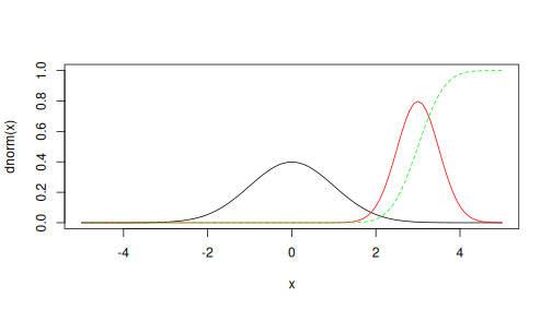

Besides norm for normal distribution, the other distribution include

• binom for binomial (and Bernoulli). It needs two parameters, sample size and probability
• lnorm for log-normal
• pois for Poisson. It requires one parameter, the expected value.
• exp for exponential
• gamma for gamma distribution. It requires a shape parameter.
• beta for beta distribution. It requires two shape parameters.

There are more built-in distribution, and add-on packages provide even more distributions.

11.2 Simulating statistical models

Random numbers are extremely useful when you want to test and try out statistical models.

11.2.1 A simple case: law of large numbers

For instance, let’s demonstrate the Law of Large Numbers–the sample average is approaching the expected value as the sample size \(N\to\infty\). In order to demonstrate this, we need to pick a random process, average of which we are analyzing. Let’s use a very simple one–flip two coins and compute the numbre of heads. Two coins can be simulated as rbinom(2, 1, 0.5), we’ll replicate this many times, and compute the average. If the number of replications \(R\) is large, the average number of heads should be close to unity.

For a given number of replications, we can code this as

1. create a vector to store the number of heads in each replication
2. for each experiment do the following:
   1. flip two fair coins using rbinom(2, 1, 0.5). This will result in two numbers, both either “0” or “1”.
   2. compute the total number of heads (just sum these numbers)
   3. save the sum into the vector
3. compute the average of the number of heads that are stored in the vector.

Thereafter we can repeat the above for different number of experiments.

Let’s do the code for 10 experiments:

S <- 2  # how many coins do you flip
R <- 10  # how many experiments
heads <- numeric(R)  # number of heads in each experiment
for(i in 1:R) {
   coins <- rbinom(S, 1, 0.5)
   heads[i] <- sum(coins)
}
heads  # show the results of every experiement

##  [1] 1 2 1 2 1 2 1 1 0 1

You can see that we’ll get mostly either 1 or 2 heads, but in one case also no heads. Finally, we are not interested in every single result but the average number of heads over experiments:

mean(heads)

## [1] 1.2

Note that these simulations involve two sample size: one, denoted by \(S\) is the number of coins, and the other, denoted by \(R\), is the number of replications–how many time do we flip \(S\) coins.

This was a single experiment with 10 replications. If we want to see how LLN works, we need to repeat it for different number of replications, e.g. from 1 to 1000, in a loop. Each time we compute the average number of heads, and we need a vector to store those averages (called avgs below):

N <- 1000  # the max # of experiments
avgs <- numeric(N)  # experiment averages
for(R in 1:N) {
   heads <- numeric(R)  # number of heads in each experiment
   for(i in 1:R) {
      coins <- rbinom(2, 1, 0.5)
      heads[i] <- sum(coins)
   }
   avgs[i] <- mean(heads)
}
head(avgs)  # just check -- take a look  at a few values 

## [1] 1.000000 1.500000 1.666667 1.000000 1.400000 1.000000

Now avgs contains the average number of heads for 1, 2, … \(R\) trials.

Finally, let’s make a plot to show how the average depends on \(R\):

plot(avgs, xlab = "R", ylab = "Average",
     type = "l")
axis(4)  # add axis on right side of the plot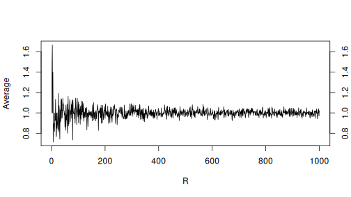

The plot shows how the initial large wobbles at small \(R\) values converge to close to one–the expected value.

11.2.2 Sample average

TBD: simulate the distribution of sample average

TBD: exercise: sample quantiles

11.2.3 Linear regression

Linear regression has a number of assumptions, one of which is that the error term is normally distributed. If the model is \[\begin{equation} y_i = \beta_0 + \beta_1 \cdot x_i + \epsilon_i \end{equation}\] then \[\begin{equation} \epsilon_i \sim N(0, \sigma^2). \end{equation}\]

Let’s make the following experiment: assume there is no relationship between \(x\) and \(y\). We sample data of size \(N\). How often do we see a relationship just because of the sample is random?

First we need to decide about the parameters \(\beta_0\) and \(\beta_1\). Assuming there is no relationship is equivalent to setting \(\beta_1 = 0\). The assumption does not say anything about \(\beta_0\) though–it is essentially average \(y\) value and we can pick any number. For simplicity, we can pick \(\beta_0 = 0\) as well.

Next, we need to specify \(x\) values. As these are not stochastic, we can, again, pick all sorts of numbers, such as 1, 2, …, 10; or just random numbers here too. Let’s imagine our data only contains numbers 1 to 10, so we can randomly sample from these as sample(10, N, replace = TRUE).

The most important step is to model the relationship between \(y\) and \(x\). As we assume there no relationship, \(y\) is just equal to the error term \(\epsilon\). But below we still use the full specification \[\begin{equation} y = \beta_0 + \beta_1 \cdot x + \epsilon \end{equation}\] for consistency, using \(\beta_0 = \beta_1 = 0\).

Assume the standard assumption is correct and the error term follows the standard normal \(\epsilon \sim N(0, 1)\). (We can also see what happens if this assumption is violated, but let’s leave this exercise for another time.)

Finally, let’s look at a small sample of size \(N = 10\). So a single dataset can be generated as

beta0 <- beta1 <- 0
N <- 10
x <- sample(10, N, replace = TRUE)
eps <- rnorm(N)
y <- beta0 + beta1*x + eps
plot(x, y)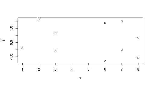

As expected, if \(\beta_1 = 0\), we do not see much of a relationship between \(x\) and \(y\). This can be confirmed with linear regression:

m <- lm(y ~ x)
summary(m)

## 
## Call:
## lm(formula = y ~ x)
## 
## Residuals:
##     Min      1Q  Median      3Q     Max 
## -1.4970 -0.9905  0.3834  0.5775  1.3023 
## 
## Coefficients:
##             Estimate Std. Error t value Pr(>|t|)
## (Intercept)  0.28616    0.70291   0.407    0.695
## x            0.02883    0.12445   0.232    0.823
## 
## Residual standard error: 1.105 on 8 degrees of freedom
## Multiple R-squared:  0.006665,   Adjusted R-squared:  -0.1175 
## F-statistic: 0.05368 on 1 and 8 DF,  p-value: 0.8226

\(\beta_1\), denoted here by x, is 0.029

But how often can we see a relationship, just because of the random nature of sampling? To answer this question, we can repeat the experiment many times, each time estimate a linear regression model, and save the estimated \(\beta_1\). What are the largest values we see there?

We can use a very similar code to what we did above. Generate data using the example above; fit a linear regression model; extract the coefficient "x", and save it in a vector:

R <- 1000
beta0 <- beta1 <- 0
N <- 10
betas <- numeric(R)
for(r in 1:R) {
   x <- sample(10, N, replace = TRUE)
   eps <- rnorm(N)
   y <- beta0 + beta1*x + eps
   m <- lm(y ~ x)
   betas[r] <- coef(m)["x"]
}
hist(betas, breaks = 30)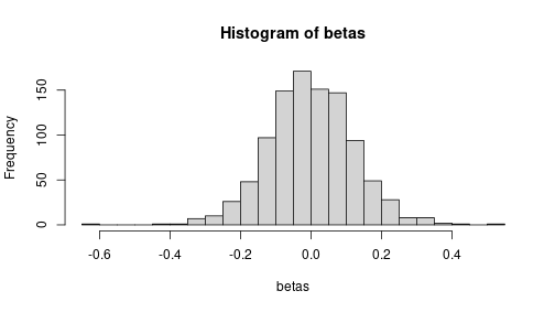

But the largest estimated values are above 0.5 (in absolute value):

range(betas)

## [1] -0.6447306  0.5119822

Even if there is no true relationship, we’ll occasionally see quite a substantial estimates–just because of random sampling.

The standard deviation of the estimated betas is very close to what we computed above:

sd(betas)

## [1] 0.1248484

This ensures that the statistics, as compute by summary() are reliable.

Exercise 11.2 The simulation above assumes that the intercept \(\beta_0 = 0\). But what happens if you choose a different \(\beta_0\), e.g. \(\beta_0 = 10\)?

1. create a single sample of data, and estimate the linear regression model as above. What is the estimated \(\beta_1\)? How big is its standard error?
2. Repeat the above 1000 times and display the histogram of estimated \(\beta_1\), and its standard deviation. Do you get numbers that are close to those in the regression summary table?
3. Explain what you find!

Exercise 11.3 The reason that your simulated standard errors are so close to the theoretical ones as provided by the summary table, is that we have fulfilled all the assumptions behind the theoretical standard errors. One of these is that the error term is normally distributed, \(\epsilon \sim N(0, \sigma^2)\). But what happens if the error term is not normally distributed?

1. Use three different distributions for the error terms:
   1. rectangular, standard uniform (\(\epsilon \sim Unif(0,1)\)). You can sample it as runif(N).
   2. Asymmetric, exponential (\(\epsilon \sim Exp(1)\)), can be simulated as rexp(N, 1)
   3. Very unequal, log-normal (\(\epsilon \sim LN(0, 1.5)\)), can be simulated as rlnorm(N, 0, 1.5)
2. replicate what we did above.
3. do the simulated results and theoretical results align?

See the solution