Chapter 3 Rmarkdown: literal programming with R
RMarkdown is the most popular approach for literal programming in R. Literal programming is a method of mixing computer code and free text, afterwards the code will be replaced by its output. This is a very handy approach for creating work notes where you can easily add long textual comments to your code and output, and for reports where the analysis part must be repeatedly recalculated as data and methods are updated.
The notes below concern rmarkdown. We do not discuss other options, such as using LaTeX instead of markdown as the textual environment around code, or running R in jupyter notebooks. While one can use any text editor to create rmarkdown files, we also limit our discussion to RStudio only.
3.1 Creating and using rmarkdown files
3.1.1 Creating rmarkdown files
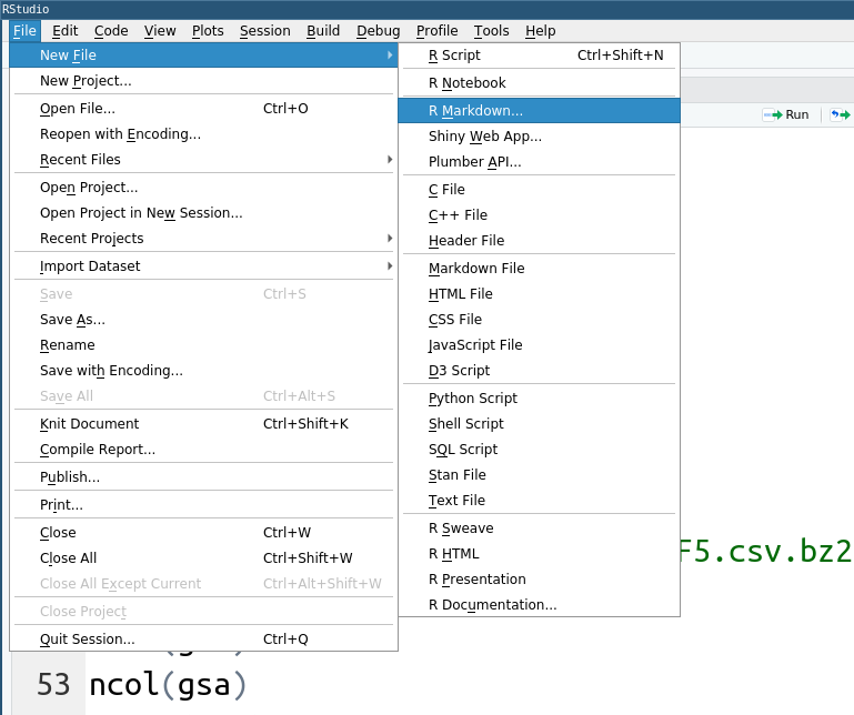
Rstudio makes it easy to create new rmarkdown files by simply selecting the appropriate items in the menu (Files → New File → R Markdown).
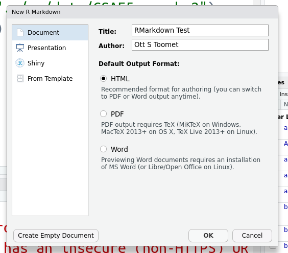
The menu brings up a dialog window that allows to choose a few basic
properties of the new document. In particular, you can give it a
title, adjust the name of author, and select the document type. The
latter determines what is the result of the compilation. Here we only
discuss HTML documents but there are many more options. All these
options (and many more) can also be adjusted later in the YAML
header in the top of the file.
Rmarkdown documents normally use .rmd or .Rmd file extension.
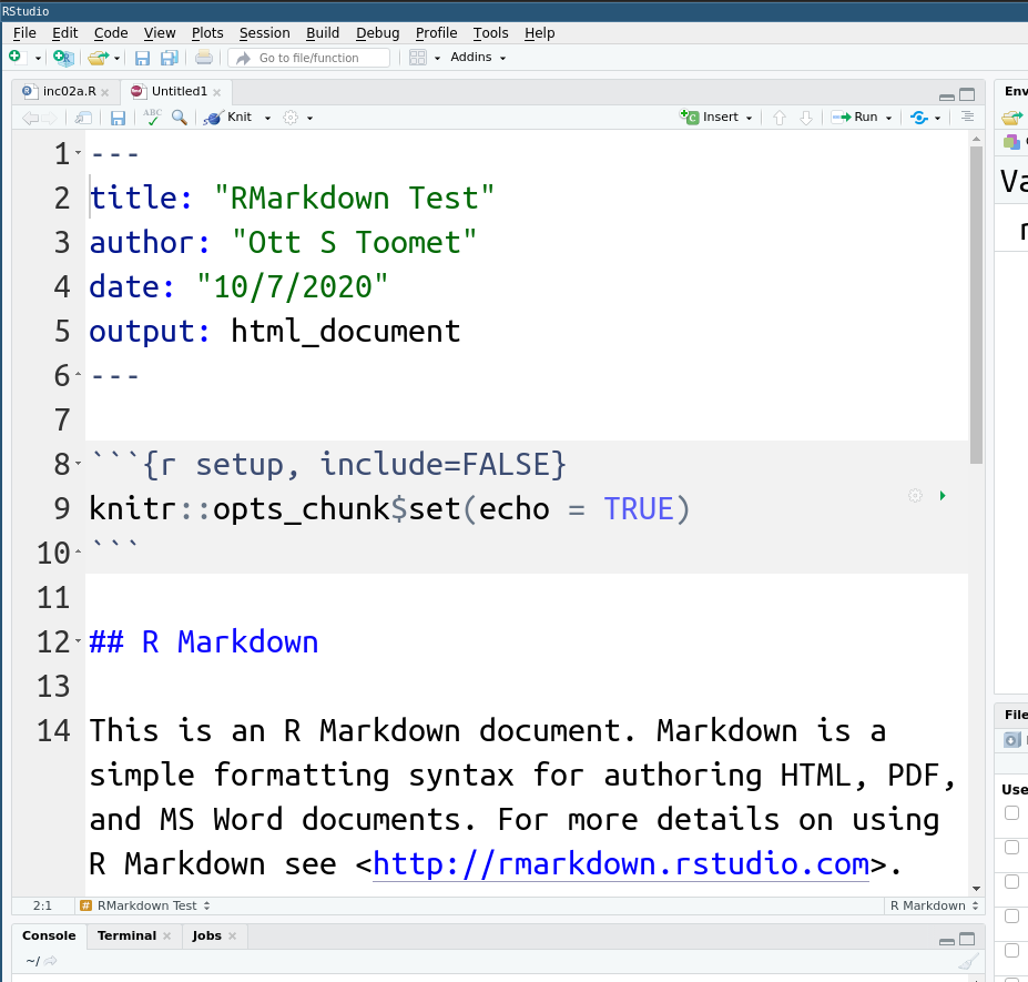
A new rmarkdown file is not empty but contains a document template. This is a valid document, you can compile it (knit it) and you will get a small explanatory page. The template serves just a basic reminder of the available options and syntax, you should to replace its content with your own text and code.
In this example one can see a code chunk, the grayed-out lines in
the middle of the image. A code chunk starts with three tick marks, followed by
{r}. The braces may also contain chunk options,
e.g. include=FALSE in the example here. Code chunk ends with three tickmarks.
In this example it is followed by normal markdown text.
3.1.2 Knitting (compiling) rmarkdown
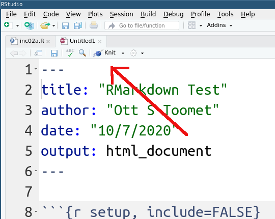
The RMarkdown document is not yet ready for prime-time. It must be compiled and rendered. This is called “knitting” and can achieved by clicking the “knit”-button. Note that there is also a simple pull-down menu next to knit button, it allows one to override the default document type. For now, let us just stay with the plain knit button and HTML documents.
You are strongly encouraged to memorize the keyboard shortcut for
knitting, e.g. Ctrl-Shift-K in linux. Hover you mouse over the
button to see the shortcut for your system.
Behind the scenes, knitting performs two tasks:
It extract all R code from the document, executes it, and creates a new document where the code is replaced with the corresponding output. This is a plain markdown document, not rmarkdown any more. Note that it does not have to be just R code, one can include various programming languages in rmarkdown documents (including julia, python and bash shell).
It uses pandoc to convert markdown document to an html page. The html document will be saved in the same folder, next to your original rmarkdown document. In case of different output format, the steps may be slightly different.
Finally, by default RStudio opens the resulting html file in its own simple browser. RStudio’s internal browser is fairly limited but good enough for a quick overview. One can switch to the full browser by clicking its “Open in browser” button.
Knitting is done in a new clean R session located in the same folder where the markdown file is located. So R code inside of markdown does not have access to the variables and data you have defined in your interactive R session. It must be explicitly loaded for the new session. Keep also in mind that your rmarkdown document may be in a different folder than what is the current working directory of your R session, so the path names may need to be adjusted accordingly.
One can also knit documents without RStudio. This needs to execute R and knitr from command line, for instance as
Rscript -e "knitr::knit2html('my-document.rmd')"There are many options for doing this, and normally you want to include this command in a makefile. This is beyond the scope of these notes, consult knitr documentation for more information. You can also consult the included makefiles in the repo of these notes.
3.1.3 R Notebooks
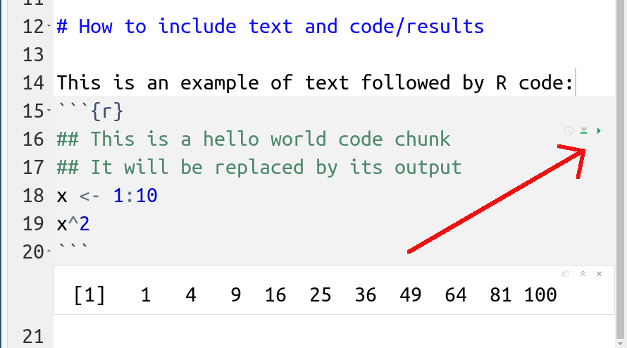
Ctrl-Shift-Enter).
Another handy way to use rmarkdown is to treat it as a notebook. Note that we are talking about rmarkdown notebooks (R notebooks) here, not about running R inside jupyter notebooks.
R notebook file itself is no different from rmarkdown, the difference
is in the way how you run it. While you may want to knit the
whole document into a single webpage as your final product, for
testing and developing purposes it is very handy to run code chunks
one-by-one and inspect their results. This can be achieved by
clicking on the small green triangle on the top-right corner of code
chunks (or even better, learn the keyboard shortcut Ctrl-Shift-Enter).
This will run the code and show its output right underneath the code
chunk (the line without the row number in the figure).
I stress here again that in terms of file format, rmarkdown and R notebook are identical, the difference is just how the code is executed.
While R notebooks (and other notebooks) are good for evaluation and testing, they have their own caveats:
- Code chunks in notebooks are typically run repeatedly and out of order, and meanwhile one modifies the code (this is why you do testing!) However, this may break the resulting markdown file when run in order from start to end. It is advisable to frequently re-knit and fix the resulting issues.
- Unlike knitting, notebooks are run in the current R session, so the code chunks have access to all variables and data loaded interactively. This also means that the working directory of the chunks is the current working directory of the R session, and if the markdown file is located in a different folder, the file loading commands may not work correctly!
Note that while you can use any text editor to write rmarkdown documents, there is limited support for running it as a notebook outside of RStudio.
We repeat the caveat with R sessions:
Knitting is done in a new R session located in the same folder where the markdown file is located. But when you run chunks as notebook then they are run inside of the current R session. In particular, the working directory for notebook and for knitting may be different!
3.2 Rmarkdown syntax
RMarkdown is just a mix of ordinary markdown with R code cunks. Markdown is a simple markup language (language to mark structure of written text), somewhat similar to HTML and Latex.
3.2.1 Markdown syntax
The most commonly used markdown structures are headers
# Title, first level header
## Second level header
### Third level
...
Text formatting:
**bold**, _italic_, **_bold italic_**for bold, italic, and bold italic text.
Web links can be inserted as [link text](link url), e.g.
[University of Washington](www.uw.edu)which results in University of Washington. Images are
essentially a special type of links in the form  where alternate text is displayed in context where
the image itself cannot be displayed. This includes screen readers,
but also when the image file is missing. The exclamation mark in
front of the image command means to load the image onto the page–if
you leave it out you will have image link instead of image.
One can display inline code formatted with special fixed width font as
text ... `code` ... more textwhich results in
text … code … more text
More extensive code chunks (or any other kind of pre-formatted text)
can be displayed with by embracing the corresponding lines between
triple ticks ```:
```
first line of code
second line of code
```
which gives
first line of code
second line of code
One can also denote the programming language and get the appropriate syntax coloring (if knitr supports the corresponding language). Compare:
```
if(x > 2) cat("large\n")
```
which gives
if(x > 2) cat("large\n")and
```r
if(x > 2) cat("large\n")
```
which results in
if(x > 2) cat("large\n")3.2.2 Code chunks
The difference between ordinary markdown and rmarkdown is the latter’s
ability to execute code chunks, and replace the code with the
corresponding output. In order to make a code chunk executable, one
has to wrap it into ```{r} and ```, for instance
```{r}
print(1:5)
```
This tells knitr that this code chunk is to be extracted from the rmarkdown document as part of R code, executed, and the result put back into the document. As a result we get
## [1] 1 2 3 4 5Alternatively, if we want to enter a single result, such as a result
of certain calculations,
into the text, we can use inline code cunks in the
form `r code`, for instance
We can compute that 1 + 1 = `r 1 + 1`This results in “we can compute that 1 + 1 = 2”.
The option to use both separate and inline code chunks makes rmarkdown quite a powerful tool to write data-heavy documents. It is possible to wrap larger calculations into separate code chunks, or separate code files, and only show the results in a normal text flow.
Note that rmarkdown (or more specifically, its compiler knitr) also supports other programming languages. Some of these are pre-defined, for instance python:
```{python}
[i**2 for i in range(5)]
```
Results in:
[i**2 for i in range(5)]## [0, 1, 4, 9, 16]You can also define additional coding languages; what is needed is mainly the command for the relevant compiler, and maybe also syntax coloring.
3.2.3 Code chunk options
The code chunks can be adjusted in a multitude of ways. This is typically done using chunk options where you add options to the code chunks like
```{r, option1=value1, option=value2, ...}
... code ...
```
Below we list a few more important ones.
3.2.3.1 Display/hide code
Code can be displayed with echo=TRUE
and hidden with echo=FALSE. For instance
```{r, echo=TRUE}
print(1:4)
```
will show both code and its output like this:
print(1:4)## [1] 1 2 3 43.2.3.2 Continue/stop on errors
One can force knitting to break with error message by using the option
error=FALSE. In contrary, when using option error=TRUE, then
knitting will continue, and the error message will be displayed in the
markdown instead. So we can create code chunks like
```{r, error=TRUE}
print(nonExistingVariable)
```
and get
print(nonExistingVariable)## Error: object 'nonExistingVariable' not foundThis is handy when doing extensive modifications in your document. The document will still knit, so you can have an overview of the result while fixing the problems later.
Unfortunately, this option does not affect the inline code chunks. So code like
The answer is `r print(nonExistingVariable)`Will still result in an error that stops the code from compiling 🙁…
Exercise 3.1 Create a new rmarkdown document. Inside it load dplyr library, but
add message = FALSE chunk option to the respective code chunk. Does
the load of startup messages go away?
3.2.3.3 Hide/display warnings and messages
Sometimes your code produces a lot of harmless but annoying warnings
and messages. These can be suppressed with warning=FALSE and
message=FALSE. For instance
```{r, warning=FALSE}
log(-1)
```
Will avoid the Warning message: In log(-1) : NaNs produced
and just print NaN:
log(-1)## [1] NaN3.2.3.4 Cache: speed up computations
One of the more advanced and very handy feature is cache. This makes knitr to save the computation result on disk. If the code chunk has not changed when you knit it again, it just loads the results from the disk and does not re-do the computations. In case of complex computations it will speed up knitting tremendously, e.g.
```{r, cache=TRUE}
x <- a_very_long_computation()
print(x)
```
The cache feature is quite complex, for instance it allows to declare dependencies between different chunks and other objects, like file modification timestamps. One can also adjust the folder where data is stored. See more in Chunk options and package options by Yihui Xie.
3.2.3.5 Set global options: knitr::opts_chunk
Finally, one can also set the default options for all chunks in the
current markdown file. This can be done using
knitr::opts_chunk$set(option1=value1, option2=value2, ...). This is
typically done very early in the rmarkdown file, such as in the first
setup chunk. For instance, let’s supress code output, warnings and
messages for all the following chunks:
```{r, echo=FALSE}
knitr::opts_chunk$set(echo=FALSE, warning=FALSE, message=FALSE)
```
All following chunks will now show no code nor warnings, unless we
request it for a particular chunk by specifying, for instance, echo=TRUE.
3.3 How to debug rmarkdown documents
Rmarkdown documents are noticeably more complex to debug than interactive R code. But there are many common errors and debugging strategies.
3.3.1 Common errors
Remember that knitting is normally run in a new separate R session that does not have access to the variables you have defined in your workspace. All variables must be defined inside the rmarkdown document (or explicitly imported therein).
The working directory of knitting is normally the directory where the rmd file is located. This may be different from your interactive R session, and hence may give you “No such file” errors.
Knitting cannot handle interactive commands. In particular,
RStudio-specific View cannot be executed in knitr. This may result
in obscure errors about your graphical system. You should use
print or cat for output. knitr::kable is another way to display
your data in a nice way.
Do not install packages inside of rmarkdown document! First, it does not work without additional configuration (setting CRAN mirror), and second, it makes knitting unnecessarily slow.
3.3.2 Debugging strategies
Ensure your code works. It is often useful to ensure that the individual code chunks work by running those interactively as R notebooks. For more complex tasks this is often the preferred way.
However, while it is useful, this approach cannot be stated as a commandment. Remember, knitting is run in its own environment in a potentially different working directory. Running the same code in two different environments adds additional complexity and potentially different bugs. So while it is useful, it is not something that you must always ensure.
Use error=TRUE chunk option. This allows knitting to finish so
you can actually see the output. Otherwise knitr may just stop
with an error message, but you do not know what did the code achieve
before running into the error.
Print intermediate results. Often the wrong final result gives you only little idea what exactly went wrong in your code. So add lines to your code that print various information about your intermediate results, e.g. how many rows of data are left after filtering, what are the file names, what is the current working directory of this R session that runs knitr, and so on.
Note that this is a more general way of debugging and not just limited to knitr.
Remove part of the code. If your code just fails with incomprehensible errors, and you cannot locate the culprit, it is often useful to remove a part of your code/text until you have isolated the lines where the problem occurs. You may work with a copy your original file and restore the original one afterward. If you work under version control then you can create a dedicated git branch for this debugging task.