A Dataset Description
Here is a brief description of the datasets that are used in this book.
A.1 House votes
In repo as house-votes-84.csv.bz2
Voting behavior of 435 representatives of the U.S. House. The data is from 1984 and contains votes for 16 bills. Columns do not have names, but they are:
- column 1: party (republican/democrat)
- columns 2-17: vote for 16 different bills. Values are “y” for year, “n” for nay and “?” if neither year nor nay was registered.
It is typically used for predicting party based on the voting behavior.
Example:
read_delim("../data/house-votes-84.csv.bz2",
           col_names = FALSE) %>%
   sample_n(4)
## # A tibble: 4 × 17
## X1 X2 X3 X4 X5 X6 X7 X8 X9 X10 X11 X12 X13
## <chr> <chr> <chr> <chr> <chr> <chr> <chr> <chr> <chr> <chr> <chr> <chr> <chr>
## 1 repub… y y n y y y n n n y n n
## 2 repub… n y n y y y n n n y y y
## 3 democ… y n y n n n y y y y n n
## 4 repub… n ? n y y y n n n n n y
## # ℹ 4 more variables: X14 <chr>, X15 <chr>, X16 <chr>, X17 <chr>A.2 Hubble
In repo as hubble.csv
Distance and radial velocity data data of 24 galaxies from the 1929 publication by E. Hubble A Relation Between Distance And Radial Velocity Among Extra-Galactic Nebulae, Proceedings of the National Academy of Sciences, 1929, 15, 168-173.
Variables are- object: name of the galaxy
- ms: magnitude (brightness) of brightest stars in that galaxy. Magnitude of a few closest objects are denoted by “..”, this is so even in the original paper.
- R: distance (Mpc)
- v: radial velocity (km/s), negative values are toward us
- mt: visual magnitude (brightness)
- Mt: absolute magnitude
- D
- Rmodern: modern distance estimate (km/s)
- vModern: modern radial velocity estimate (km/s)
The modern estimates are obtained from wikipedia.
Data example:
hubble <- read_delim("../data/hubble.csv")
hubble %>%
   sample_n(4)
## # A tibble: 4 × 9
## object ms R v mt Mt D Rmodern vModern
## <chr> <chr> <dbl> <dbl> <dbl> <dbl> <dbl> <dbl> <dbl>
## 1 7331 19 1.1 500 10.4 -14.8 1.1 12.2 816
## 2 4736 17.3 0.5 290 8.4 -15.1 0.5 4.91 308
## 3 4472 .. 2 850 8.8 -17.7 2 17.1 998.
## 4 598 .. 0.263 -70 7 -15.1 0.26 0.84 -179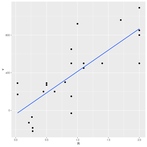
Hubble diagram, based on his 1929 data.
The data was used for the famous Hubble diagram (Figure 1 in the 1929 paper):
hubble %>%
   ggplot(aes(R, v)) +
   geom_point(size = 2) +
   geom_smooth(method = "lm",
               se = FALSE)
(The original figure corrects for solar motion though.)
A.3 Iris
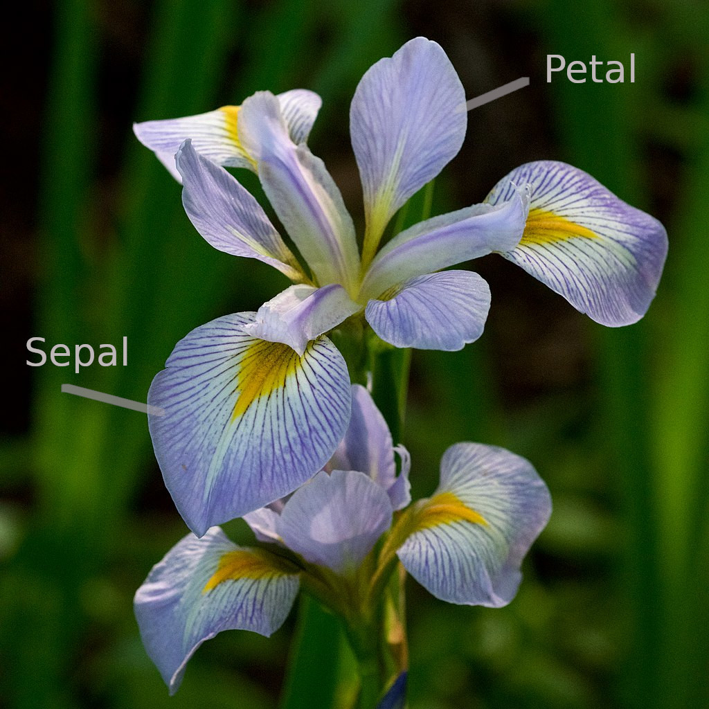
Virginica flower. The image shows large sepals and smaller petals. Sepals typically function as support and cover for flowers in bud and are green, while petals are brightly colored to attract pollinators. Iris flowers, however, have both types of leaves colored in a similar fashion.
Source: Eric Hunt, CC BY-SA 4.0, via Wikimedia Commons.
Iris dataset is collected by Ronald Fisher 1936. It contains sepal and petal measures (see the figure for explanation) of 150 iris flowers of three species–setosa, versicolor and virginica (50 of each).
It is an R built-in dataset and can be loaded with
data(iris)The variables are
- Sepal.Length: sepal length, in cm
- Sepal.Width
- Petal.Length
- Petal.Width
- Species: setosa/versicolor/virginica
The widths and lengths are measured with precision of one millimeter, and hence there are quite a few overlapping values.
Data example:
iris %>%
   sample_n(4)
## Sepal.Length Sepal.Width Petal.Length Petal.Width Species
## 1 5.0 3.4 1.5 0.2 setosa
## 2 6.0 3.4 4.5 1.6 versicolor
## 3 5.7 2.8 4.1 1.3 versicolor
## 4 5.2 3.4 1.4 0.2 setosaA.4 Orange trees
In repo as orange-trees.csv
Orange tree size (circumference) as a function of age for five different trees.
This is a version of R built-in dataset Orange. However, it is stored as csv file in order to enforce the tree id to be an integer.
Variables:
- tree: tree id (1-5)
- age: in days (days since 1968/12/31)
- circumference: trunk circumferences (mm). This is probably “circumference at breast height”, a standard measurement in forestry.
Data example:
orange <- read_delim("../data/orange-trees.csv")
orange %>%
   slice(c(1,2, 8,9))
## # A tibble: 4 × 3
## tree age circumference
## <dbl> <dbl> <dbl>
## 1 1 118 30
## 2 1 484 58
## 3 2 118 33
## 4 2 484 69A.5 Titanic
In repo as titanic.csv.bz2.
List of RMS Titanic passengers, their name, age and some more data, and whether they survived the shipwreck. It was collected by the investigation committee, and contains most of the passengers on the boat. The dataset is available in various sources, e.g. at kaggle. The variables are
- pclass Passenger Class (1 = 1st; 2 = 2nd; 3 = 3rd)
- survived Survival (0 = No; 1 = Yes)
- name Name
- sex Sex
- age Age
- sibsp Number of Siblings/Spouses Aboard
- parch Number of Parents/Children Aboard
- ticket Ticket Number
- fare Passenger Fare
- cabin Cabin
- embarked Port of Embarkation (C = Cherbourg; Q = Queenstown; S = Southampton)
- boat Lifeboat code (if survived)
- body Body number (if did not survive and body was recovered)
- home.dest The home/final destination of passenger
Example:
titanic <- read_delim("../data/titanic.csv.bz2")
titanic %>%
   sample_n(4)
## # A tibble: 4 × 14
## pclass survived name sex age sibsp parch ticket fare cabin embarked
## <dbl> <dbl> <chr> <chr> <dbl> <dbl> <dbl> <chr> <dbl> <chr> <chr>
## 1 3 1 Dowdell, … fema… 30 0 0 364516 12.5 <NA> S
## 2 1 0 Fry, Mr. … male NA 0 0 112058 0 B102 S
## 3 3 0 Mineff, M… male 24 0 0 349233 7.90 <NA> S
## 4 3 0 Bourke, M… male 40 1 1 364849 15.5 <NA> Q
## # ℹ 3 more variables: boat <chr>, body <dbl>, home.dest <chr>A.6 Treatment
In repo as treatment.csv.bz2. Originates from R package Ecdat. A U.S. dataset from 1974, used for evaluating treatment effect of training on earnings.
- treat: treated, participated in the job training program (TRUE/FALSE)
- age: age
- educ: education in years
- ethn: three categories: “other”, “black”, “hispanic”
- married: married (TRUE/FALSE)
- re74: real annual earnings in 1974 (USD, pre-treatment)
- re75: real annual earnings in 1975 (USD, pre-treatment)
- re78: real annual earnings in 1978 (USD, post-treatment)
- u74: unemployed in 1974 (TRUE/FALSE)
- u75: unemployed in 1975 (TRUE/FALSE)
Example
treatment <- read_delim("../data/treatment.csv.bz2")
treatment %>%
   sample_n(5)
## # A tibble: 5 × 10
## treat age educ ethn married re74 re75 re78 u74 u75
## <lgl> <dbl> <dbl> <chr> <lgl> <dbl> <dbl> <dbl> <lgl> <lgl>
## 1 FALSE 22 13 other FALSE 7739. 3760. 16255 FALSE FALSE
## 2 FALSE 34 16 other TRUE 35267. 34016. 35465. FALSE FALSE
## 3 FALSE 50 7 black TRUE 13715. 12532. 16255 FALSE FALSE
## 4 FALSE 45 17 other TRUE 0 16113. 17733. FALSE TRUE
## 5 FALSE 26 8 other TRUE 8151. 7448. 9901. FALSE FALSEA.7 Yin-yang
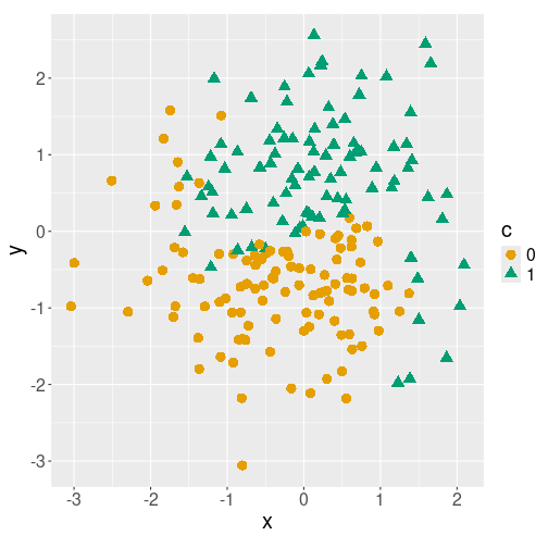
Classes 0 and 1 plotted with different colors/symbols on the plane.
- x, y: location on plane (both between about -3 and 3)
- c: category, 0/1
Example:
yinyang %>%
   head(4)
## # A tibble: 4 × 3
## x y c
## <dbl> <dbl> <fct>
## 1 -1.63 0.584 0
## 2 0.624 -0.113 0
## 3 -0.688 1.74 1
## 4 0.391 1.13 1