Chapter 13 Prediction and Predictive Modeling
Up to now we were discussing the inferential modeling. The main purpose for that approach is to learn something about the data and the world behind it. Now our focus will shift to predictive modeling–models that predict the data as well as possible. If these models also tell us something about the deeper relationship is of secondary importance.
13.1 Manually predicting regression outcomes
Manual prediction is usually not needed. It is useful though for better understanding of the underlying models, and sometimes for debugging.
13.1.1 Linear regression
Linear regression predictions are fairly simple to be reproduced manually.
13.1.1.1 Hubble data example
Let’s use an example of Hubble data, but this time predict distance based on velocity, and use the moder estimates Rmodern and vModern.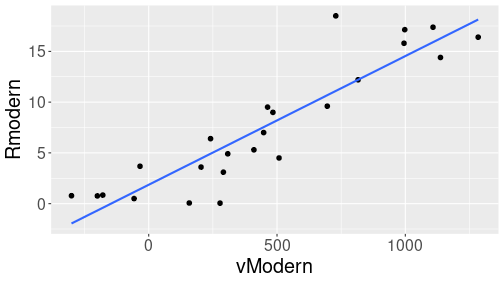
The distance-velocity relationship is shown here.
hubble <- read_delim("../data/hubble.csv")
hubble %>%
   ggplot(aes(vModern, Rmodern)) +
   geom_point(size = 2) +
   geom_smooth(method = "lm",
               se = FALSE)
Below, we are using different modeling tools to make predictions, based on this relationship, formally written as \[\begin{equation} R_i^{\mathit{Modern}} = \beta_0 + \beta_1 \cdot v_i^{\mathit{Modern}} + \epsilon_i. \end{equation}\]
Note that this is technically a very easy case as this does not include any categorical variables. If these are needed, then we need first to convert categoricals to dummies, and use the dummies instead.
13.1.1.2 Doing predictions
Before we can start with predictions, we need to find the intercept
\(\beta_0\) and slope \(\beta_1\). This is best to be done with the
lm() function of base-R (see Section 12.1.3.1):
m <- lm(Rmodern ~ vModern, data = hubble)The estimated parameter values are
coef(m)## (Intercept) vModern
## 1.86177763 0.01267665For simplicity, let’s extract the intercept and slope, and call those
b0 and b1 respectively:
b0 <- coef(m)[1]
b1 <- coef(m)[2]
Finally, we can just plug these values in to predict distance \(\hat R\): \[\begin{equation} \hat{R} = \hat{\beta}_0 + \hat{\beta_1} \cdot v \end{equation}\] where \(\hat{\beta}_0\) and \(\hat{\beta}_1\) denote the coefficient we calculated above. For instance, for the first 3 galaxies in the dataset, we can compute the predicted distance as
b0 + b1 * hubble$vModern[1:3]## [1] 3.865956 5.385886 1.139209Alternatively, if we have velocity measurements 500, 1000, and 2000 km/2, we can compute the predicted distance as
v <- c(500, 1000, 1500)
b0 + b1 * v
## [1] 8.200102 14.538426 20.87675113.1.2 Logistic regression
In case of logistic regression, we can predict both probability of outcome (called \(\hat P\) or phat below) and outcome category (called \(\hat y\) or yhat below). Logistic regression is somewhat more complex to work with manually.
13.1.2.1 Titanic data example
Below we do an example, using Titanic data. We model survival as a function of age only, as the other two main predictors (sex and pclass) are categorical and hence hard to handle for manual work. So we are fitting a logistic regression model \[\begin{equation} \Pr(S = 1) = \Lambda \big( {\beta}_0 + {\beta_1} \cdot \mathit{age} \big) = \Lambda(\eta) \end{equation}\] where \[\begin{equation} \eta = {\beta}_0 + {\beta_1} \cdot \mathit{age} \end{equation}\] is the link function, \[\begin{equation} \Lambda(\eta) = \frac{1}{1 + \exp(-\eta)} \end{equation}\] is the logistic function (aka sigmoid function) and \(s = 1\) denotes that the passenger survived.
First we fit the model:
titanic <- read_delim("../data/titanic.csv.bz2") %>%
   filter(!is.na(age))  # many age's missing
m <- glm(survived ~ age, family = binomial, data = titanic)
This commands compute the best \(\beta_0\) and \(\beta_1\), here
coef(m)## (Intercept) age
## -0.136531206 -0.007898598b0 <- coef(m)[1]
b1 <- coef(m)[2]13.1.2.2 Predicting probabilities
From above, we can estimate the survival probability of passengers as7
eta <- b0 + b1*titanic$age
phat <- 1/(1 + exp(-eta))
## print for first 3 passengers:
phat[1:3]
## [1] 0.4096069 0.4641188 0.4619914All these numbers are less than 0.5, so all of these passengers were predicted more likely to die than to survive.
Here we should stop for a moment and ask how do we know that the
probabilities above are survival probabilities, not death
probabilities? This is related to how the outcome variable survived
is coded. Here it is coded as “0” for death and “1” for survival, and
glm will predict probability of “1”. If the response variable were
coded as text, the values are converted to categorical (using
factor() function), this normally makes the alphabetically first
value to be considered as failure, and second one as “success”. For
instance, if instead of “0” and “1”, the codes were “no boat” and
“boat” (for drowning and surviving), the “boat” would be considered
failure and “no boat” success. See ?gml and ?factor.
If we need to predict probabilities for certain passengers who were, for instance, 10, 30, and 50 years old, we can achieve this as
age <- c(10, 30, 50)
eta <- b0 + b1*age
phat <- 1/(1 + exp(-eta))
phat
## [1] 0.4463283 0.4076982 0.370176213.1.2.3 Predicting categories
Sometimes probabilities are all we want, but other times we want a “yes” or “no” answer–was someone predicted to survive or die?
The basics is quite easy: we normally predict success if the probability of “success” is larger than probability of “failure”. Here, in case of two categories only, this is equivalent to predict success if predicted \(\Pr(S = 1) > 0.5\):
yhat <- phat > 0.5
yhat
## [1] FALSE FALSE FALSEWe predicted “FALSE” for all these example persons, hence all of them were predicted to die.
Again, you need to be aware what “success” and “failure” mean here. If you are interested to recover the original categories, I’d recommend to write it like this:
ifelse(phat > 0.5, 1, 0) # all predicted to die## [1] 0 0 0Manual predictions.
Linear regression
Predict outcomes:
yhat <- b0 + b1*xLogistic regression
Predict probabilities:
eta <- b0 + b1*age
phat <- 1/(1 + exp(-eta))
Predict categories:
yhat <- phat > 0.5 # TRUE/FALSE13.2 Base R modeling tools
Base-R offers a pretty good modeling framework. The central tool for predicting model outcomes is the predict method. It has two important arguments, the fitted model, and potentially also the new data. There are more arguments for certain types of models, e.g. in case of logistic regression it is possible to predict more outcomes than just the outcome probability.
13.2.1 Linear regression
Here we replicate the example from Section 13.1.1.2 using the base-R modeling tools. First fit the linear regression model:
m <- lm(Rmodern ~ vModern, data = hubble)The central tool for making predictions from a fitted model is the
function predict(). Its first argument is the model. For instance,
we can get the distance for the first 3 galaxies in the data as
predict(m)[1:3]## 1 2 3
## 3.865956 5.385886 1.139209You can check that the results are exactly the same as in Section 13.1.1.2.
Alternatively, if we want to predict the distance to galaxies that are not in the original dataset we used for fitting the model, we can create a new data frame with these measurements, and supply it as an additional argument newdata to the predict function. For instance,
newdata <- data.frame(vModern = c(500, 1000, 1500))
predict(m, newdata = newdata)
## 1 2 3
## 8.200102 14.538426 20.876751Again, these results are exactly the same as in Section 13.1.1.2.
Note that the new data frame must contain all variables that are
used in the model (here vModern). It may contain more columns but
those are just ignored.
13.2.2 Logistic regression
For logistic regression, predict() works in a fairly
similar fashion as in case of linear regression. However, now we have
to tell predict() what exactly to predict using the argument
type. The default option,
predict the link \(\eta\), is of little use. So to predict the survival
probability for everyone on Titanic, you can use
m <- glm(survived ~ age, family = binomial, data = titanic)
phat <- predict(m, type = "response")  # 'response' is probability
phat[1:3]  # first 3 probabilities
## 1 2 3
## 0.4096069 0.4641188 0.4619914These numbers are exactly the same as above in Section
13.1.2.2. In case we want to predict
survival for a person who is not in the original dataset, we need to
supply a data frame with the newdata argument, see above in Section
13.2.1.
Predict for glm() does not do categories–if you need categories
instead of probabilities, you need to follow the steps in Section
13.1.2.3. For instance,
yhat <- phat > 0.5  # TRUE/FALSE
yhat[1:3]
## 1 2 3
## FALSE FALSE FALSEifelse(phat > 0.5, 1, 0)[1:3] # 1/0## 1 2 3
## 0 0 0Exercise 13.1
Use Titanic data.- Include only age. Fit the model, predict the survival probabilities, and plot a histogram of those. (30 bins is a good when plotting the histogram).
- Instead of just age, include six age groups: 0-5, 6-12, 13-18, 19-34, 35-55, 56- (see Section 6.2.1). Predict survival probability and plot the histogram. Why does the histogram have very few bars only?
- Now include age groups, sex, and their interactions (see Section 12.1.4).
- Include also pclass (as categorical, see Section 12.1.4), and its interactions with sex.
- Take your model 3. Which groups are predicted to have very high
and very low survival probabilities? Predict the probability for a
- 5 year old girl;
- 30 year old woman;
- 5 year old boy;
- 30 year old man.
Bare-R predictions.
Linear regression
Predict outcomes:
predict(m)
predict(m, newdata = nd)
Logistic regression
Predict categories:
phat <- predict(m, type = "response")Predict categories:
yhat <- phat > 0.5 # TRUE/FALSE13.3 Using tidymodels
The modeling tools in base-R are mainly developed with inferential modeling in mind. But R also has several frameworks that are dedicated for predictive modeling. Such packages typically provide a more unified interface for models that are commonly used in prediction, the model assessment tools, such as confusion matrix and other model goodness measures, and tools to optimize parameters in pipelines. Unfortunately, as the tasks are different, so are different the tools, and hence bring a substantial learning curve.
This section discusses predictions using one of such frameworks, namely the tidymodels package. It is a package that works well together with tidyverse, but you need to install and load it separately:
library(tidymodels)13.3.1 Basic modeling
First, we discuss the basics of modeling with tidymodels. Its approach is heavily based on pipes, but unlike in case of dplyr, it is not data that flows through the pipe from function to function–it is the model that flows through fitting and prediction steps.
13.3.1.1 Linear regression
As the first step, let’s replicate the task in Section 13.1.1.1, predicting the distance of galaxies by their speed, using tidymodels.
First, we define the model:
m <- linear_reg()This creates an empty linear regression model m. If has no defined parameters and it has no defined formulas. It is just an empty model that one can fit (or use in pipelines, see Section 15).
Next, we fit the model with a data, using a formula:
mf <- m %>%
   fit(Rmodern ~ vModern, data = hubble)
Note how the pipe forwards not data (which is given as a separate
argument) but the model into the fit() function.
fit() creates a new object, a fitted model, that we can use for
different tasks. For instance, here is a tidy-style version of the
regression table:
tidy(mf)## # A tibble: 2 × 5
## term estimate std.error statistic p.value
## <chr> <dbl> <dbl> <dbl> <dbl>
## 1 (Intercept) 1.86 0.799 2.33 0.0294
## 2 vModern 0.0127 0.00127 9.96 0.00000000130This is the exact same table as one can get using the base-R lm()
and summary() methods, just printed in a slightly different way.
For instance, the \(t\)-values are called statistic instead.
Unfortunately, summary(mf) does not produce anything meaningful with
fitted model objects.
Predicting with tidymodels works in a fairly similar way as with the base-R tools. Here is an example how we can use the model to predict the distance of two galaxies, with speeds 500 and 1500 km/2:
newData <- data.frame(vModern = c(500, 1500))
predict(mf, new_data = newData)
## # A tibble: 2 × 1
## .pred
## <dbl>
## 1 8.20
## 2 20.9You can see two differences–the new data argument is called new_data, and more importantly, the result is a data frame where the column of predictions is called .pred (remember–it is a vector in base-R).
There is another important difference–the new_data argument is required (in base-R, if you leave it out, then the model predicts for the original data). It is not that common in predictive modeling to predict on the training data, so this difference is understandable. But here is how you can do it:
predict(mf, new_data = hubble) %>%
   sample_n(4)
## # A tibble: 4 × 1
## .pred
## <dbl>
## 1 7.73
## 2 4.45
## 3 10.7
## 4 4.9213.3.1.2 Logistic regression
Let’s demonstrate tidymodels approach with a classification problem. The basic workflow is very similar.
First we define the model, this time it is logistic_reg():
m <- logistic_reg()And next, you need to fit it. logistic_reg() requires the outcome
variable to be categorical, so we need to use factor(survived)
instead of just survived:
mf <- m %>%
   fit(factor(survived) ~ factor(pclass) + sex, data = titanic)
As in case of the linear regression, the coefficient table (not the
marginal effects!) can be extracted with tidy().
But predicting probabilities and outcomes is much more straightforward
with tidymodels. Both of these will be computed by predict(mf, new_data = ...). In order to get probabilities, we need to add type = "prob":
predict(mf, new_data = titanic,
                # new data required
                # compute for everyone
        type = "prob") %>%
                # predict probability
   head(3)
## # A tibble: 3 × 2
## .pred_0 .pred_1
## <dbl> <dbl>
## 1 0.103 0.897
## 2 0.591 0.409
## 3 0.103 0.897This returns a data frame with two columns: .pred_0 and .pred_1.
These are predicted probabilities for drowning (survived = 0) and
surviving (survived = 1). For instance, the first passenger is
predicted to survive with probability 0.897 while the 2nd one has
survival chances of only 0.409.
We can also predict the class directly by specifying type = "class"
(or by just leaving it out):
predict(mf, type = "class",
                           # can leave type out as well
        new_data = titanic) %>%
                           # new data required!
   head(3)
## # A tibble: 3 × 1
## .pred_class
## <fct>
## 1 1
## 2 0
## 3 1This, again, produces a data frame with a single column,
.pred_class. And indeed, we can see that the first passenger is
predicted to survive while the second one to die.
Finally, a small example about how to predict the outcome for new cases, here for a 1st class man and a second class women. We have specified age as well, but the model is not using it.
newData <- data.frame(sex = c("male", "female"),
                      pclass = c(1, 2),
                      age = c(10, 20))
predict(mf, new_data = newData)
## # A tibble: 2 × 1
## .pred_class
## <fct>
## 1 0
## 2 1 # no 'type' argument -> predict classInstead of writing
phat <- 1/(1 + exp(-eta))below, one can use the logistic probability functionplogis()asphat <- plogis(eta).↩︎