Chapter 15 Machine Learning Workflow
This section describes typical machine learning workflows–fitting the model, computing its performance, tinkering with it, and trying over again. This is how you determine which model is the best, and what hyperparameter values to use.
Obviously, ML involves many more tasks, in particular data cleaning and pre-processing, but we do not discuss it here.
First we provide the examples using base-R, and afterwards show how to achieve the related results using tidymodels.
15.1 Overfitting: random numbers improve results!
This section demonstrates many of the relevant tools by overfitting a classification (logistic regression) model. We do it by adding random data to the model. As random numbers are not related to the data and outcomes, they should not change the results. In particular, they should not substantially improve the results. However, if we assess the model performance on the training data, then the model’s performance will actually improve.
15.1.1 The baseline model
Below is an example using House votes data. We’ll use
First we load it and give the columns meaningful names:
hv <- read_delim("../data/house-votes-84.csv.bz2",
                 col_names = c("party", paste0("v", 1:16)))
head(hv, 3)
## # A tibble: 3 × 17
## party v1 v2 v3 v4 v5 v6 v7 v8 v9 v10 v11 v12
## <chr> <chr> <chr> <chr> <chr> <chr> <chr> <chr> <chr> <chr> <chr> <chr> <chr>
## 1 republican n y n y y y n n n y ? y
## 2 republican n y n y y y n n n n n y
## 3 democrat ? y y ? y y n n n n y n
## v13 v14 v15 v16
## <chr> <chr> <chr> <chr>
## 1 y y n y
## 2 y y n ?
## 3 y y n nNext, for simplicity, let’s only use data about the first 4 votes, and
convert it (either “y”, “n” or “?”)
into a logical variable with TRUE for yea, FALSE for
non-yea. We’ll aso convert party into republican (true/false):
hv <- hv %>%
   select(party, v1:v4) %>%
                           # only 4 first votes for simplicity
   mutate(across(v1:v4, function(x) x == "y"),
          republican = party == "republican") %>%
   select(!party)
head(hv, 3)
## # A tibble: 3 × 5
## v1 v2 v3 v4 republican
## <lgl> <lgl> <lgl> <lgl> <lgl>
## 1 FALSE TRUE FALSE TRUE TRUE
## 2 FALSE TRUE FALSE TRUE TRUE
## 3 FALSE TRUE TRUE FALSE FALSEAs the last step in data preparation, I extract the column party as the outcome vector y. We do not need it here, but will make the notation simpler below.
y <- hv$republicanAs this is a classification problem, we use logistic regression. First model republican using the four votes:
m <- glm(republican ~ ., family = binomial(), data=hv)and thereafter predict:
yhat <- predict(m, type="response") > 0.5As we do not have preferences over type-1/type-2 errors, we can just use accuracy to evaluate the model:
acc <- mean(yhat == y)
acc
## [1] 0.9494253So the model gets roughly 94.9 percent of the predictions right.
15.1.2 Adding random columns to data
Next, let’s add a column of random TRUE/FALSE-s to the data. Here we
use sample() to pick the correct number of TRUE-s and FALSE-s:
r <- sample(c(TRUE, FALSE), nrow(hv), replace=TRUE)
               # the random column
hv1 <- cbind(hv, r)
Now there is an additional, random column, in the updated data frame hv1:
hv1 %>%
   sample_n(3)
## v1 v2 v3 v4 republican r
## 1 FALSE TRUE FALSE TRUE TRUE FALSE
## 2 TRUE TRUE FALSE TRUE TRUE FALSE
## 3 TRUE FALSE TRUE FALSE FALSE TRUEWe fit a similar model, this time also including the random column:
m <- glm(republican ~ ., family="binomial", data=hv1)
yhat <- predict(m, type="response") > 0.5
acc1 <- mean(y == yhat)
acc1
## [1] 0.9563218This resulted in a slightly better accuracy, the difference is 0.69 percentage points.
If we add more random columns, the results will improve even more. Here an example with 10 columns:
r10 <- sample(c(TRUE, FALSE), 10*nrow(hv), replace=TRUE) %>%
               # create random T/F for 10 columns
   matrix(ncol=10) %>%
               # transform it to a 10-column matrix
   as.data.frame()
               # and into a 10-column data frame
hv10 <- cbind(hv, r10)
m <- glm(republican ~ ., family="binomial", data=hv10)
yhat <- predict(m, type="response") > 0.5
acc10 <- mean(y == yhat)
acc10
## [1] 0.9609195Now the accuracy is 96.09, an improvement of 1.15 percentage points.
If we add enough random data, we’ll eventually get perfect predictions:
r40 <- sample(c(TRUE, FALSE), 40*nrow(hv), replace=TRUE) %>%
               # 40 columns of random data
   matrix(ncol=40) %>%
   as.data.frame()
hv40 <- cbind(hv, r40)
m <- glm(republican ~ ., family="binomial", data=hv40)
## Warning: glm.fit: algorithm did not converge## Warning: glm.fit: fitted probabilities numerically 0 or 1 occurredyhat <- predict(m, type="response") > 0.5
mean(y == yhat)## [1] 1We’ll get convergence warnings, but the accuracy is now 1–adding enough random data will give us perfect results.
15.2 Training-validation split
We should compute model performance on validation data, not training data:
iTrain <- sample(nrow(hv), 0.8*nrow(hv))
hvTrain <- hv[iTrain,]
hvValid <- hv[-iTrain,]
For a check, let’s see the dimensions:
dim(hvTrain)## [1] 348 5dim(hvValid)## [1] 87 5The original data is split between 348 training and 87 validation cases, roughly in 80/20 ratio.
m <- glm(republican ~ ., family = binomial, data=hvTrain)
yhat <- predict(m, type="response", newdata=hvValid) > 0.5
mean(y == yhat)
## [1] 0.5172414The performance on the training data in the original form is similar to performance on the complete data.
Now see how the performance looks like if we add random columns:
hvTrain <- hv100[iTrain,]
hvValid <- hv100[-iTrain,]
yTrain <- hv$republican[iTrain]
yValid <- hv$republican[-iTrain]
m <- glm(republican ~ ., family="binomial", data=hvTrain)
## Warning: glm.fit: algorithm did not converge## Warning: glm.fit: fitted probabilities numerically 0 or 1 occurredyhat <- predict(m, type="response", newdata=hvValid) > 0.5
mean(yValid == yhat)## [1] 0.9310345Now the performance is noticeably less–only 90%.
We can see how the performance of the model changes if we continue adding random columns. We can just loop over number of columns and just continue adding random columns:
rcolumns <- seq(1, 350, by=5)
aTrain <- aValid <- numeric()
iTrain <- sample(nrow(hv), 0.8*nrow(hv))
i <- 1
for(rcols in rcolumns) {
   r <- sample(c(TRUE, FALSE), rcols*nrow(hv), replace=TRUE) %>%
      matrix(ncol=rcols)
   X <- cbind(hv, r)
   XTrain <- X[iTrain,]
   XValid <- X[-iTrain,]
   yTrain <- y[iTrain]
   yValid <- y[-iTrain]
   m <- glm(republican ~ ., family = binomial(),
            data = XTrain)
   yhat <- predict(m, type="response") > 0.5
   aTrain[i] <- mean(yTrain == yhat)
   yhat <- predict(m, type = "response", newdata = XValid) > 0.5
   aValid[i] <- mean(yValid == yhat)
   i <- i + 1
}
data.frame(rcolumns, aTrain, aValid) %>%
   head(6)
## rcolumns aTrain aValid
## 1 1 0.9511494 0.9310345
## 2 6 0.9655172 0.9310345
## 3 11 0.9655172 0.9655172
## 4 16 0.9885057 0.9425287
## 5 21 0.9741379 0.9540230
## 6 26 1.0000000 0.9195402Finally, let’s plot these results:
plot(rcolumns, aValid, type="l",
     xlab="# of random columns", ylab="Accuracy",
     ylim=c(0,1))
legend("bottomleft",
       legend=c("Training", "Validation"),
       lty=1, col=c("black", "red"))
lines(rcolumns, aTrain, col="red")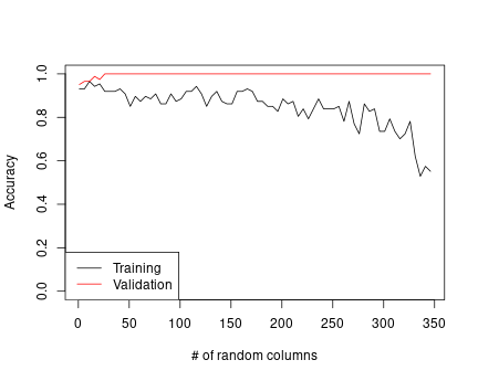
15.3 tidymodels workflow
For more advanced usage, it is common not to build such training and validation pipelines yourself, but to use ready-made packages.
library(tidymodels)Below, we demonstrate this using the tidymodels approach, using decision trees. However, trees work better if we use more columns than just the first four votes (otherwise tree depth will not influence the results, as the trees will always and only rely on vote 4).
hv <- read_delim("../data/house-votes-84.csv.bz2",
                 col_names = c("party", paste0("v", 1:16)))
hv <- hv %>%
   mutate(across(v1:v16, function(x) x == "y"),
          republican = factor(party == "republican")) %>%
                           # classification tree requires a factor outcome
   select(!party)
y <- hv$republican
Training-validation split
splitData <- validation_split(hv, prop = 0.80)## Warning: `validation_split()` was deprecated in rsample 1.2.0.
## ℹ Please use `initial_validation_split()` instead.
## This warning is displayed once every 8 hours.
## Call `lifecycle::last_lifecycle_warnings()` to see where this warning was generated.m <- decision_tree(mode = "classification",
tree_depth = tune(),
cost_complexity = 1e-5,
min_n = 3)recipe <- recipe(republican ~ ., data = hv)wf <- workflow() %>%
add_model(m) %>%
add_recipe(recipe)
wf## ══ Workflow ════════════════════════════════════════════════════════════════════════════════════════════════════════
## Preprocessor: Recipe
## Model: decision_tree()
##
## ── Preprocessor ────────────────────────────────────────────────────────────────────────────────────────────────────
## 0 Recipe Steps
##
## ── Model ───────────────────────────────────────────────────────────────────────────────────────────────────────────
## Decision Tree Model Specification (classification)
##
## Main Arguments:
## cost_complexity = 1e-05
## tree_depth = tune()
## min_n = 3
##
## Computational engine: rpartgrid <- data.frame(tree_depth = 1:5)
grid## tree_depth
## 1 1
## 2 2
## 3 3
## 4 4
## 5 5res <- wf %>%
tune_grid(splitData,
grid = grid,
control = control_grid(save_pred = TRUE),
metrics = metric_set(accuracy,
precision, recall, f_meas)
)res## # Tuning results
## # Validation Set Split (0.8/0.2)
## # A tibble: 1 × 5
## splits id .metrics .notes .predictions
## <list> <chr> <list> <list> <list>
## 1 <split [348/87]> validation <tibble [20 × 5]> <tibble [0 × 3]> <tibble [435 × 5]>metrics <- res %>%
collect_metrics()
filter(metrics, .metric == "accuracy")## # A tibble: 5 × 7
## tree_depth .metric .estimator mean n std_err .config
## <int> <chr> <chr> <dbl> <int> <dbl> <chr>
## 1 1 accuracy binary 0.954 1 NA Preprocessor1_Model1
## 2 2 accuracy binary 0.954 1 NA Preprocessor1_Model2
## 3 3 accuracy binary 0.966 1 NA Preprocessor1_Model3
## 4 4 accuracy binary 0.954 1 NA Preprocessor1_Model4
## 5 5 accuracy binary 0.966 1 NA Preprocessor1_Model5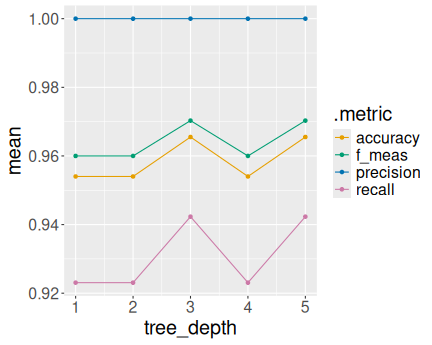
Different metrics as a function of tree depth
For better understanding, let’s plot how do the performance indicators depend on the tree depth:
ggplot(metrics,
       aes(tree_depth, mean, col = .metric)) +
   geom_point() +
   geom_line()