B Solutions
B.1 R Language
B.1.1 Operators
B.1.1.1 Create vectors
Using operators and sequences:
v <- 1:5
v^2
## [1] 1 4 9 16 25or you can do it just as
(1:5)^2## [1] 1 4 9 16 25Using c:
c(1,4,9,16,25)## [1] 1 4 9 16 25B.1.1.2 Going out with friends
friends <- 7
budget <- 150
cat("I am going out with", friends, "friends\n")
## I am going out with 7 friendsmealprice <- 14
price <- mealprice*(friends + 1)
total <- price*1.15
cat("total price:", total, "\n")## total price: 128.8if(total <= budget) {
cat("can afford\n")
} else {
cat("cannot afford\n")
}## can affordB.2 Pipes and dplyr
B.2.2 dplyr
B.2.2.1 Select Titanic variables
## one way
titanic %>%
   select(pclass, survived, sex, age) %>%
   head(2)
## pclass survived sex age
## 1 1 1 female 29.0000
## 2 1 1 male 0.9167## another way
titanic %>%
select(pclass:age & !name) %>%
head(2)## pclass survived sex age
## 1 1 1 female 29.0000
## 2 1 1 male 0.9167Note combining two criteria with logical and & in the second example.
for the following answers we need the subset of babynames data:
babynames <- babynames::babynames %>%
   select(-prop) %>%
   filter(between(year, 1995, 2003))
B.2.2.2 Longest name
We can just compute the length of the names, arrange by the length in descending order, and pick the first names:
babynames %>%
   mutate(len = nchar(name)) %>%
   group_by(sex) %>%
   arrange(desc(nchar(name)), by_group=TRUE) %>%
   slice_head(n=3)
## # A tibble: 6 × 5
## # Groups: sex [2]
## year sex name n len
## <dbl> <chr> <chr> <int> <int>
## 1 1997 F Hannahelizabeth 5 15
## 2 1995 F Mariaguadalupe 21 14
## 3 1995 F Mariadelcarmen 11 14
## 4 1995 M Johnchristopher 13 15
## 5 1995 M Christopherjame 9 15
## 6 1995 M Franciscojavier 8 15This results in longest names printed for both boys and girls.
Alternatively, we can use min_rank to implicitly order the names,
and pick the names with rank 1:
babynames %>%
   group_by(sex) %>%
   filter(min_rank(desc(nchar(name))) == 1)
## # A tibble: 48 × 4
## # Groups: sex [2]
## year sex name n
## <dbl> <chr> <chr> <int>
## 1 1995 M Johnchristopher 13
## 2 1995 M Christopherjame 9
## 3 1995 M Franciscojavier 8
## 4 1995 M Christiandaniel 7
## 5 1995 M Christopherjohn 6
## 6 1995 M Jonathanmichael 6
## 7 1996 M Franciscojavier 13
## 8 1996 M Jonathanmichael 9
## 9 1996 M Christopherjohn 8
## 10 1996 M Christophermich 8
## 11 1996 M Christopherjose 7
## 12 1996 M Christiananthon 6
## 13 1996 M Christianmichae 6
## 14 1996 M Christianjoseph 5
## 15 1996 M Christopherjame 5
## 16 1996 M Davidchristophe 5
## 17 1996 M Jordanchristoph 5
## 18 1996 M Ryanchristopher 5
## 19 1997 F Hannahelizabeth 5
## 20 1997 M Christophermich 8
## 21 1997 M Johnchristopher 8
## 22 1997 M Franciscojavier 7
## 23 1997 M Ryanchristopher 7
## 24 1997 M Christopherjame 6
## 25 1997 M Christopherjohn 6
## 26 1997 M Christopherryan 5
## 27 1998 M Christopherjame 12
## 28 1998 M Christopherjohn 9
## # ℹ 20 more rowsWe can see that there are quite a few 15-character long names, apparently compound names. But we also see another problem–names are counted multiple times if they appear in multiple years. In order to solve that problem, we may group by name and sex, and sum over n, before we check the name length:
babynames %>%
   group_by(name, sex) %>%
   summarize(n = sum(n)) %>%
   group_by(sex) %>%
   filter(min_rank(desc(nchar(name))) == 1)
## # A tibble: 19 × 3
## # Groups: sex [2]
## name sex n
## <chr> <chr> <int>
## 1 Christiananthon M 12
## 2 Christiandaniel M 7
## 3 Christianjoseph M 10
## 4 Christianjoshua M 5
## 5 Christianmichae M 6
## 6 Christopheranth M 6
## 7 Christopherjame M 45
## 8 Christopherjohn M 39
## 9 Christopherjose M 12
## 10 Christophermich M 16
## 11 Christopherryan M 5
## 12 Davidchristophe M 5
## 13 Franciscojavier M 52
## 14 Hannahelizabeth F 5
## 15 Johnchristopher M 39
## 16 Jonathanmichael M 20
## 17 Jordanchristoph M 5
## 18 Matthewalexande M 11
## 19 Ryanchristopher M 22This table lists 19 names, all of these 15 letters long. Interestingly, only one of these was given to girls. It appears that 15 letters is the limit in this dataset, e.g. Christianmichae is probably either Christianmichael or more likely Christian Michael.
B.3 Cleaning data
B.3.1 Missing values
B.3.1.1 Use na_if and filtering
We use na_if to convert empty strings to NA-s and thereafter
remove all explicit missings:
titanic %>%
   mutate(boat = na_if(boat, "")) %>%
   filter(!is.na(boat)) %>%
   nrow()
## [1] 486This is exactly the same number as in Section 6.1.2.
B.3.1.2 Replace missing value in ice extent data
First (re)create the data:
extent <- data.frame(month=9:12, extent=c(7.28, 9.05, 11.22, -9999))
extent
## month extent
## 1 9 7.28
## 2 10 9.05
## 3 11 11.22
## 4 12 -9999.00- Obviously, missing is coded as
-9999. As extent is a measure of area, it cannot be negative, so even if documentation is not there, we can conclude that the value is invalid, and we should replace it. - Convert it to
NA:
extent %>%
   mutate(extent = na_if(extent, -9999))
## month extent
## 1 9 7.28
## 2 10 9.05
## 3 11 11.22
## 4 12 NA- use the previous value with
tidyr::fill. Previous values will be used when `.direction = “down”:
extent %>%
   mutate(extent = na_if(extent, -9999)) %>%
   fill(extent, .direction="down")
## month extent
## 1 9 7.28
## 2 10 9.05
## 3 11 11.22
## 4 12 11.22B.4 ggplot
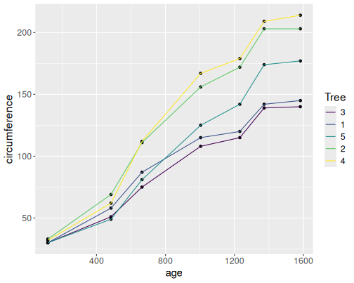
B.4.0.1 Orange trees as scatterplots
data(Orange)
Orange %>%
   ggplot(aes(age, circumference, col=Tree)) +
   geom_point()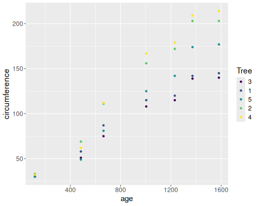
B.5 Statistics
B.5.2 Simulating statistical models
B.5.2.1 Expected value, variance of functions of RV
Theoretical values:
- \(\mathbb{E} X = -10 \cdot 0.1 + 0 \cdot 0.5 + 1 \cdot 0.4 = -0.6\)
- \(\mathrm{Var}X\): it is easier to use the shortcut formula \[\begin{equation*} \mathrm{Var}X = \mathbb{E}X^2 - (\mathbb{E} X)^2 \end{equation*}\] So need to compute \[\begin{equation*} \mathbb{E} X^2 = 100 \cdot 0.1 + 0 \cdot 0.5 + 1 \cdot 0.4 = 10.4. \end{equation*}\] Hence \[\begin{equation*} \mathrm{Var}X = 10.4 - 0.6^2 = 10.04 \end{equation*}\]
- \[\begin{align*} \mathbb{E} \mathrm{e}^X &= \mathrm{e}^{-10} \cdot 0.1 + \mathrm{e}^{0} \cdot 0.5 + \mathrm{e}^{1} \cdot 0.4 =\\&= 0.00005 \cdot 0.1 + 1 \cdot 0.5 + 2.7183 \cdot 0.4 =\\&= 1.587 \end{align*}\]
- For variance, we need to compute \[\begin{align*} \mathbb{E} (\mathrm{e}^X)^2 &= \mathrm{e}^{-20} \cdot 0.1 + \mathrm{e}^{0} \cdot 0.5 + \mathrm{e}^{2} \cdot 0.4 =\\&= 0 \cdot 0.1 + 1 \cdot 0.5 + 7.3891 \cdot 0.4 =\\&= 3.456 \end{align*}\] and hence the variance \[\begin{equation*} \mathrm{Var}X = \mathbb{E}X^2 - (\mathbb{E} X)^2 = 0.936 \end{equation*}\]
Simulations:
## Create the sample
x <- sample(c(-10, 0, 1), 10000,
            prob = c(0.1, 0.5, 0.4),
            replace = TRUE)
## EX
mean(x)
## [1] -0.5985## Var X
var(x)## [1] 10.09931## E e^X
mean(exp(x))## [1] 1.597986## Var e^X
var(exp(x))## [1] 0.943186All simulated figures are close to the theoretical values.
B.5.2.2 Linear regression with wrong error terms
First, here with uniform distribution. The code is identical to the example in Section 11.2.3, except we replace the distribution:
beta0 <- beta1 <- 0
N <- 10
x <- sample(10, N, replace = TRUE)
eps <- runif(N)
y <- beta0 + beta1*x + eps
summary(m <- lm(y ~ x))
##
## Call:
## lm(formula = y ~ x)
##
## Residuals:
## Min 1Q Median 3Q Max
## -0.45209 -0.26165 -0.04387 0.21716 0.54237
##
## Coefficients:
## Estimate Std. Error t value Pr(>|t|)
## (Intercept) 0.4580303 0.2724789 1.681 0.131
## x -0.0002804 0.0480181 -0.006 0.995
##
## Residual standard error: 0.3449 on 8 degrees of freedom
## Multiple R-squared: 4.263e-06, Adjusted R-squared: -0.125
## F-statistic: 3.411e-05 on 1 and 8 DF, p-value: 0.9955The summary results are also similar to what we saw in Section 11.2.3. But the standard deviation of \(\beta_1\) is different, this is because standard uniform has different variance compared to the standard normal.
R <- 1000
beta0 <- beta1 <- 0
N <- 10
betas <- numeric(R)
for(r in 1:R) {
   x <- sample(10, N, replace = TRUE)
   eps <- runif(N)
   y <- beta0 + beta1*x + eps
   m <- lm(y ~ x)
   betas[r] <- coef(m)["x"]
}
hist(betas, breaks = 30)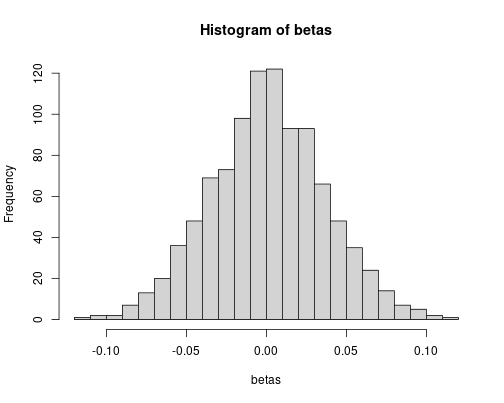
sd(betas)## [1] 0.0356941But even if the numbers are different, the simulated and theoretical values match very well.
Next, exponential distribution. Again, the code is almost identical:
beta0 <- beta1 <- 0
N <- 10
x <- sample(10, N, replace = TRUE)
eps <- rexp(N, 1)
y <- beta0 + beta1*x + eps
summary(m <- lm(y ~ x))
##
## Call:
## lm(formula = y ~ x)
##
## Residuals:
## Min 1Q Median 3Q Max
## -1.3056 -1.2619 -0.9822 -0.4143 7.5181
##
## Coefficients:
## Estimate Std. Error t value Pr(>|t|)
## (Intercept) 1.98849 2.22614 0.893 0.398
## x -0.08599 0.38348 -0.224 0.828
##
## Residual standard error: 2.872 on 8 degrees of freedom
## Multiple R-squared: 0.006247, Adjusted R-squared: -0.118
## F-statistic: 0.05029 on 1 and 8 DF, p-value: 0.8282The standard deviation is a little different, again.
R <- 1000
beta0 <- beta1 <- 0
N <- 10
betas <- numeric(R)
for(r in 1:R) {
   x <- sample(10, N, replace = TRUE)
   eps <- rexp(N, 1)
   y <- beta0 + beta1*x + eps
   m <- lm(y ~ x)
   betas[r] <- coef(m)["x"]
}
hist(betas, breaks = 30)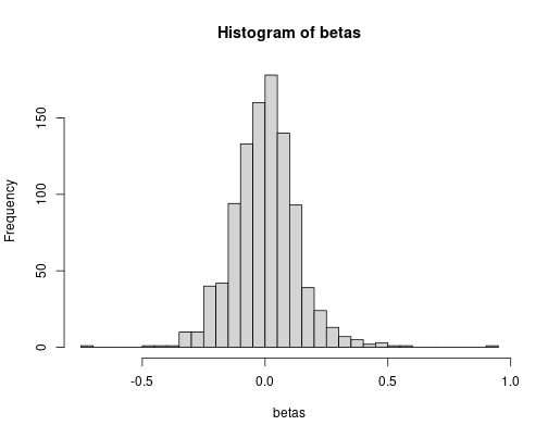
sd(betas)## [1] 0.1337823The simulated and theoretical standard deviations agree, more-or-less, although the discrepancy is a bit larger now.
Finally, highly unequal log-normal distribution:
beta0 <- beta1 <- 0
N <- 10
x <- sample(10, N, replace = TRUE)
eps <- rlnorm(N, 0, 1.5)
y <- beta0 + beta1*x + eps
summary(m <- lm(y ~ x))
##
## Call:
## lm(formula = y ~ x)
##
## Residuals:
## Min 1Q Median 3Q Max
## -1.1791 -0.6673 -0.3742 0.1466 2.6634
##
## Coefficients:
## Estimate Std. Error t value Pr(>|t|)
## (Intercept) 1.31025 1.00846 1.299 0.230
## x -0.07388 0.15067 -0.490 0.637
##
## Residual standard error: 1.202 on 8 degrees of freedom
## Multiple R-squared: 0.02918, Adjusted R-squared: -0.09217
## F-statistic: 0.2404 on 1 and 8 DF, p-value: 0.6371The estimated standard deviation is much larger now
R <- 1000
beta0 <- beta1 <- 0
N <- 10
betas <- numeric(R)
for(r in 1:R) {
   x <- sample(10, N, replace = TRUE)
   eps <- rlnorm(N, 0, 1.5)
   y <- beta0 + beta1*x + eps
   m <- lm(y ~ x)
   betas[r] <- coef(m)["x"]
}
hist(betas, breaks = 60)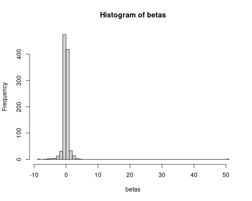
sd(betas)## [1] 1.806747But the simulated standard deviation is much larger.
Introducing very skewed distribution for the error term makes linear regression to underestimate the standard deviation and hence overestimate \(t\)-values. The statistical inference may be wrong.
B.6 Regression models
B.6.1 Linear Regression
B.6.1.1 Manually find the best virginica petal parameters
Load data
data(iris)
virginica <- iris %>%
   filter(Species == "virginica")
x <- virginica$Petal.Length
y <- virginica$Petal.Width
Define the function:
sse <- function(b0, b1) {
   yHat <- b0 + b1*x
   sum((y - yHat)^2)
}
Now start from the best value got above, \((-0.1, 0.4)\) and manipulate \(\beta_1\):
sse(-0.1, 0.4)## [1] 4.6196sse(-0.1, 0.3)## [1] 14.2024sse(-0.1, 0.5)## [1] 26.16Out of these values, \((-0.1, 0.4)\) is the best combination. Now manipulate \(\beta_0\):
sse(-0.2, 0.4)## [1] 4.1716sse(-0.3, 0.4)## [1] 4.7236The best value is \((-0.2, 0.4)\). Next, manipulate \(\beta_1\) again, just now in smaller steps:
sse(-0.2, 0.39)## [1] 4.284536sse(-0.2, 0.41)## [1] 4.369896We cannot beat \((-0.2, 0.40)\). Hence change \(\beta_0\) again:
sse(-0.19, 0.40)## [1] 4.1714sse(-0.21, 0.40)## [1] 4.1818sse(-0.18, 0.40)## [1] 4.1812Out of these, \((-0.19, 0.40)\) is the best option.
We can keep going like that, each time making the step smaller. At the end, it will lead to the correct linear regression result.
B.6.1.2 Manually optimize virginica sepal regression
We essentially follow the same example as what we did where we optimized petals manually.
First, load data and define \(x\) and \(y\):
data(iris)
virginica <- iris %>%
   filter(Species == "virginica")
x <- virginica$Sepal.Length
y <- virginica$Sepal.Width
We use the same sse function as above:
sse <- function(b0, b1) {
   yHat <- b0 + b1*x
   sum((y - yHat)^2)
}
Start with certain \((\beta_0, \beta_1)\) values $(0, 0.5) with a similar reasoning \(\beta_0 = 0\) means zero-length leaves are of zero width, and \(\beta_1 = 0.5\) means that 1cm longer leaves are 0.5cm wider. Both are a reasonable starting point:
sse(0, 0.5) # a## [1] 10.575Next, let’s try make \(\beta_1\) smaller–if it helps:
sse(0, 0.4) # b## [1] 10.33The new result, 10.33, is only a little bit better than the previous one, but it is still better.
As a third attempt, we set \(\beta_0 = -0.1\) while keeping our previous best value \(\beta_1 = 0.4\)
sse(-0.1, 0.4) # c## [1] 14.218This resulted in a worse outcome that \(\beta_0 = 0\), hence lets try the other way around in increase \(\beta_0\) to 0.1:
sse(0.1, 0.4) # d## [1] 7.442Now we get a better result, so we can move even further into the positive direction:
sse(0.2, 0.4) # e## [1] 5.554We see an additional improvement, although smaller than earlier. Let’s continue:
sse(0.3, 0.4) # f## [1] 4.666Now we got \(SSE\) below 5!
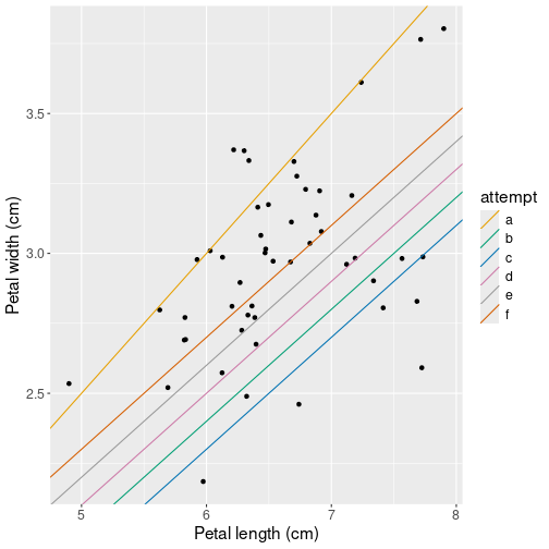
Finally, plot data and all the attempts:
## Create data frame of the three attempted parameters
lines <- data.frame(
   ## 'letters' are lowers case letters
   attempt = letters[1:6],
   intercept = c(0, 0, -0.1, 0.1, 0.2, 0.3),
   slope = c(0.5, 0.4, 0.4, 0.4, 0.4, 0.4))
## add predicted lines to the original scatterplot:
ggplot(virginica,
       aes(Sepal.Length, Sepal.Width)) +
   geom_jitter() +
   labs(x = "Petal length (cm)",
        y = "Petal width (cm)") +
   geom_abline(data=lines,
               aes(intercept=intercept,
                   slope=slope,
                   col=attempt))
We use pre-defined variable letters to label the attempts, it is
simply a vector of 26 English lower-case letters.
B.6.1.3 Titanic pclass as number and categorical
First, use pclass as a number:
lm(survived ~ pclass + sex, data = titanic) %>%
   summary()
##
## Call:
## lm(formula = survived ~ pclass + sex, data = titanic)
##
## Residuals:
## Min 1Q Median 3Q Max
## -0.8952 -0.2451 -0.0998 0.2501 0.9002
##
## Coefficients:
## Estimate Std. Error t value Pr(>|t|)
## (Intercept) 1.04054 0.03369 30.89 <2e-16 ***
## pclass -0.14531 0.01313 -11.07 <2e-16 ***
## sexmale -0.50481 0.02297 -21.98 <2e-16 ***
## ---
## Signif. codes: 0 '***' 0.001 '**' 0.01 '*' 0.05 '.' 0.1 ' ' 1
##
## Residual standard error: 0.3948 on 1306 degrees of freedom
## Multiple R-squared: 0.3413, Adjusted R-squared: 0.3403
## F-statistic: 338.3 on 2 and 1306 DF, p-value: < 2.2e-16The intercept here means that 0-class women had survival probability 1.04. This is out of range of possible probabilities, and artifact of linear probability models, but we also did not have 0-class passengers.
pclass estimate -0.14 means that passengers in one unit larger class had 14 pct points lower probability to survive.
Next, convert pclass to a factor:
lm(survived ~ factor(pclass) + sex,
   data = titanic) %>%
   summary()
##
## Call:
## lm(formula = survived ~ factor(pclass) + sex, data = titanic)
##
## Residuals:
## Min 1Q Median 3Q Max
## -0.8990 -0.2364 -0.1015 0.2587 0.8985
##
## Coefficients:
## Estimate Std. Error t value Pr(>|t|)
## (Intercept) 0.89898 0.02540 35.398 < 2e-16 ***
## factor(pclass)2 -0.15771 0.03237 -4.872 1.24e-06 ***
## factor(pclass)3 -0.29264 0.02671 -10.957 < 2e-16 ***
## sexmale -0.50487 0.02298 -21.974 < 2e-16 ***
## ---
## Signif. codes: 0 '***' 0.001 '**' 0.01 '*' 0.05 '.' 0.1 ' ' 1
##
## Residual standard error: 0.3949 on 1305 degrees of freedom
## Multiple R-squared: 0.3414, Adjusted R-squared: 0.3399
## F-statistic: 225.5 on 3 and 1305 DF, p-value: < 2.2e-16Here the reference category is 1st class females, the intercept tells that their survival probability was 0.90. 2nd class passengers had 15 pct pt lower probability to survive, and 3rd class passengers had 29 pct pt lower probability to survive.
Treating pclass as a number and as a categorical gives fairly similar results here because, for some reason, the survival probability differs by about equal amount between 1st and 2nd, and between 2nd and 3rd class passengers. In general, it is not so though.
B.6.1.4 Log age instead of age
This is just about replacing age with log(age) in the formula:
treatment <- read_delim("../data/treatment.csv.bz2")
treatment %>%
   filter(re78 > 0) %>%
   lm(log(re78) ~ educ + log(age),
      data = .) %>%
   summary()
##
## Call:
## lm(formula = log(re78) ~ educ + log(age), data = .)
##
## Residuals:
## Min 1Q Median 3Q Max
## -5.5702 -0.2372 0.1301 0.4290 2.1656
##
## Coefficients:
## Estimate Std. Error t value Pr(>|t|)
## (Intercept) 6.097644 0.195998 31.11 <2e-16 ***
## educ 0.110124 0.005101 21.59 <2e-16 ***
## log(age) 0.688133 0.050924 13.51 <2e-16 ***
## ---
## Signif. codes: 0 '***' 0.001 '**' 0.01 '*' 0.05 '.' 0.1 ' ' 1
##
## Residual standard error: 0.7399 on 2341 degrees of freedom
## Multiple R-squared: 0.1979, Adjusted R-squared: 0.1972
## F-statistic: 288.8 on 2 and 2341 DF, p-value: < 2.2e-16Now the \(R^2\) is 0.1979, originally it was 0.1908. Hence it improved the model a little bit.
B.7 Prediction and predictive modeling
B.7.1 Base-R modeling tools
B.7.1.1 Titanic predicted probabilities
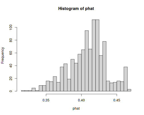
- Only age to explain survival:
m <- glm(survived ~ age,
         family = binomial,
         data = titanic)
phat <- predict(m, type = "response")
hist(phat, breaks = 30)
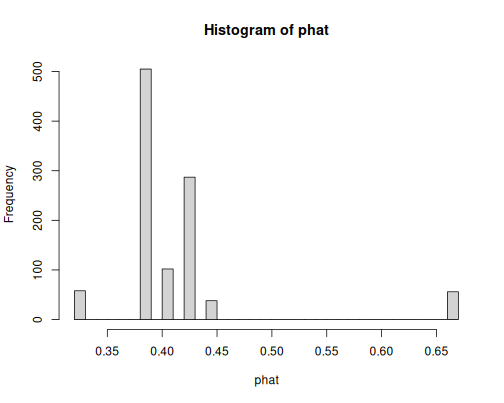
As you see, the predicted probabilities are around 0.4, this means the model has little idea if the persons survived or not. Age alone does not tell much about survival.
- Age groups
m <- titanic %>%
   mutate(
      ageGroup = cut(
         age,
         breaks = c(0, 5.5, 12.5, 18.5,
                    34.5, 55.5, Inf))) %>%
   glm(survived ~ ageGroup,
       family = binomial, data = .)
phat <- predict(m, type = "response")
hist(phat, breaks = 30)
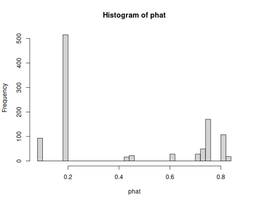
As we only have six age groups as the sole explanatory variable, the model can only predict six different probability values. One can guess that the highest bar, around 0.7, is about young children.
- Age groups, sex, and their interactions
m <- titanic %>%
   mutate(
      ageGroup = cut(
         age,
         breaks = c(0, 5.5, 12.5, 18.5,
                    34.5, 55.5, Inf))) %>%
   glm(survived ~ ageGroup*sex,
       family = binomial, data = .)
phat <- predict(m, type = "response")
hist(phat, breaks = 30)
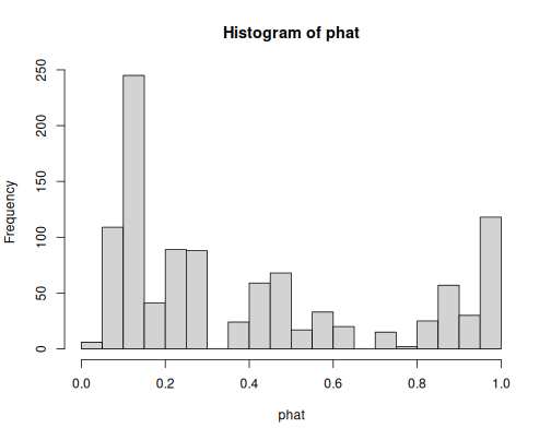
Now the predicted probabilities have more values, some of which are fairly large (above 0.8), some fairly small (less than 0.2). So the model is more confident in its predictions. One can guess that the bars around 0.8 denote women, and those below 0.2 men.
- Age groups, sex, pclass, and interactions
m <- titanic %>%
   mutate(
      ageGroup = cut(
         age,
         breaks = c(0, 5.5, 12.5, 18.5,
                    34.5, 55.5, Inf))) %>%
   glm(survived ~ ageGroup*sex +
          sex*pclass,
       family = binomial, data = .)
phat <- predict(m, type = "response")
hist(phat, breaks = 30)
We have even more values. Importantly, the distribution is now clearly bimodal, with the small values (around 0.1) and large values (around 0.9-1) dominating the picture. The model is fairly certain in many cases.
- Predicted probabilities. We need to a) fit the model; b) create a data frame that contains the four interesting cases; c) convert the age in the new data frame in exactly the same way as when modeling; and d) predict on the new data frame.
## Fit the model
m <- titanic %>%
   mutate(
      ageGroup = cut(age,
                     breaks = c(0, 5.5, 12.5, 18.5, 34.5, 55.5, Inf))) %>%
   glm(survived ~ ageGroup*sex,
       family = binomial, data = .)
## Create the data frame with desired characteristics
newdata <- data.frame(age = c(5, 30, 5, 30),
                      sex = c("female", "female",
                              "male", "male")) %>%
   ## Convert age
   mutate(ageGroup = cut(age,
                         breaks = c(0, 5.5, 12.5, 18.5, 34.5, 55.5, Inf)))
## Predict on desired data
predict(m, type = "response", newdata = newdata)
## 1 2 3 4
## 0.7142857 0.7470588 0.6071429 0.1940299So the girls have somewhat larger probability to survive than boys (0.7 versus 0.6), but adult women have even better chances (0.74). Men are at bottom with 0.19.
B.8 Assessing model goodness
B.8.1 Confusion matrix
B.8.1.1 Yin-yang decision boundary with quadratic terms
To simplify the repetitive tasks, let’s make a function for decision boundary plot:
dbplot <- function(m, nGrid = 100) {
   ex <- seq(min(yinyang$x), max(yinyang$x), length.out=nGrid)
   ey <- seq(min(yinyang$y), max(yinyang$y), length.out=nGrid)
   grid <- expand.grid(x = ex, y = ey)
   grid$chat <- predict(m, newdata = grid, type = "response") > 0.5
   ggplot() +
      geom_tile(data = grid,
                aes(x, y, fill = chat),
                alpha = 0.15) +
      geom_point(data = yinyang,
                 aes(x, y, col = c, pch = c),
                 size = 3) +
      theme(legend.position = "none") +
      coord_fixed()
}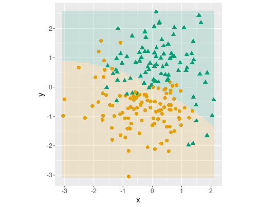
Logistic decision boundary with three terms: \(x\), \(y\) and \(x^2\).
First, only include \(x^2\):
m <- glm(c ~ x + y +
            I(x^2),
         family = binomial(),
         data = yinyang)
dbplot(m)
Logistic decision boundary with three terms: \(x\), \(y\), \(x^2\) and \(y^2\).
Second, only include both \(x^2\) and \(y^2\):
m <- glm(c ~ x + y +
            I(x^2) + I(y^2),
         family = binomial(),
         data = yinyang)
dbplot(m)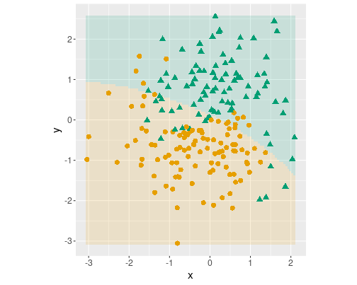
Logistic decision boundary with three terms: \(x\), \(y\), \(x^2\), \(y^2\) and \(x\cdot y\).
Finally, only include \(x^2\), \(y^2\) and \(x\cdot y\):
m <- glm(c ~ x + y +
            I(x^2) + I(y^2) + I(x*y),
         family = binomial(),
         data = yinyang)
dbplot(m)
As you can see, all three decision boundaries are almost identical. Adding more than a single quadratic term to the model makes little difference.
B.8.1.2 Decision boundary instead of decision regions
We’ll do the modelin in the same way as in Section 14.2.2. Let’s also add a quadratic term to the model in order to make the decision boundary curved:
library(tidymodels)
m <- logistic_reg() %>%
   fit(c ~ x + y + I(x*y), data = yinyang)
Thereafter we do predictions on the grid in the same way:
nGrid <- 100  # 100x100 grid
ex <- seq(min(yinyang$x), max(yinyang$x), length.out=nGrid)
ey <- seq(min(yinyang$y), max(yinyang$y), length.out=nGrid)
grid <- expand.grid(x = ex, y = ey)
## Add the predicted value to the 'grid' data frame>
grid$chat <- predict(m, type = "class",
                     new_data = grid) %>%
   pull(.pred_class)
This results in predicted values like
sample(grid$chat, 10)## [1] 1 0 1 0 1 1 0 0 0 1
## Levels: 0 1Note that these values are categories, not numbers. We can transform these to numbers, and then plot the contour line for value 0.5. You can transform the factors to numbers as (see Section 2.5.1.1):
grid <- grid %>%
   mutate(chat = as.numeric(as.character(chat)))
And now we can plot the contour line instead of geom_tile() as
ggplot() +
geom_contour(data = grid,
aes(x, y, z = chat),
breaks = 0.5) +
geom_point(data = yinyang,
aes(x, y, col = c, pch = c),
size = 3) +
theme(legend.position = "none") +
coord_fixed()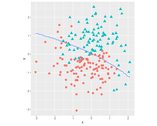 The blue line–the boundary–is
a bit zig-zaggy because of the finite
resolution of the grid.
B.8.1.3 Treatment and age with base-R tools
The initial model
treatment <- read_delim("../data/treatment.csv.bz2")
m <- glm(treat ~ age, family = binomial(),
         data = treatment)
## Predict category
yhat <- predict(m, type = "response") > 0.5
## construct CM
table(Predicted = yhat, Actual = treatment$treat)
## Actual
## Predicted FALSE TRUE
## FALSE 2490 185The cm only contains a single row (labeled FALSE). This is because the model predicts that no-one participates.
Accuracy is simple:
mean(yhat == treatment$treat)## [1] 0.9308411Recall is obviously 0: we do not identify any cases of actual participation. It can still be computed as
sum(yhat == 1 & treatment$treat == 1)/sum(treatment$treat == 1)## [1] 0But precision is undefined: 0 cases out of 0 predictions are correct. This number cannot even be calculated.
Add more variables
m <- glm(treat ~ age + ethn + u74 + u75 + re75,
         family = binomial(),
         data = treatment)
## Warning: glm.fit: fitted probabilities numerically 0 or 1
## occurred## Predict category
yhat <- predict(m, type = "response") > 0.5
## construct CM
table(Predicted = yhat, Actual = treatment$treat)## Actual
## Predicted FALSE TRUE
## FALSE 2469 63
## TRUE 21 122Now the table has all four entries–we predict some persons to participate and some not to participate.
Accuracy:
mean(yhat == treatment$treat)## [1] 0.9685981Recall:
re <- sum(yhat == 1 & treatment$treat == 1)/sum(treatment$treat == 1)
re
## [1] 0.6594595Precision:
pr <- sum(yhat == 1 & treatment$treat == 1)/sum(yhat == 1)
pr
## [1] 0.8531469Precision is larger than recall, this means the model does not capture that many participants, but those persons it predicts as participants are mostly correct.
B.8.1.4 Treatment and age with tidymodels
The initial model
library(tidymodels)
treatment <- treatment %>%
   mutate(y = factor(treatment$treat))
                           # oucome needs to be a factor
m <- logistic_reg() %>%
   fit(y ~ age, data = treatment)
yhat <- predict(m, new_data = treatment)
## Combine actual, predicted into a single df
## call them 'y' and 'yhat'
res <- yhat %>%
   cbind(y = treatment$y) %>%
   rename(yhat = .pred_class)
res %>%
   conf_mat(y, yhat)
## Truth
## Prediction FALSE TRUE
## FALSE 2490 185
## TRUE 0 0Unlike in case of the base-R table(), this cm contains both rows,
for FALSE and TRUE, although the latter is filled with zeros as
the model predicts that no-one participates.
Accuracy can be computed as:
res %>%
   accuracy(y, yhat)
## # A tibble: 1 × 3
## .metric .estimator .estimate
## <chr> <chr> <dbl>
## 1 accuracy binary 0.931but it may be easier to use the previous approach. Recall:
res %>%
   recall(y, yhat, event_level = "second")
## # A tibble: 1 × 3
## .metric .estimator .estimate
## <chr> <chr> <dbl>
## 1 recall binary 0Precision is undefined, and will result in a warning and NA:
res %>%
   precision(y, yhat, event_level = "second")
## Warning: While computing binary `precision()`, no predicted events were detected
## (i.e. `true_positive + false_positive = 0`).
## Precision is undefined in this case, and `NA` will be returned.
## Note that 185 true event(s) actually occurred for the problematic event
## level, TRUE## # A tibble: 1 × 3
## .metric .estimator .estimate
## <chr> <chr> <dbl>
## 1 precision binary NAAdd more variables
m <- logistic_reg() %>%
   fit(y ~ age + ethn + u74 + u75 + re75, data = treatment)
## Warning: glm.fit: fitted probabilities numerically 0 or 1
## occurredyhat <- predict(m, new_data = treatment)
res <- yhat %>%
cbind(y = treatment$y) %>%
rename(yhat = .pred_class)
res %>%
conf_mat(y, yhat)## Truth
## Prediction FALSE TRUE
## FALSE 2469 63
## TRUE 21 122Now all the four cells of the table contain positive values.
Accuracy:
res %>%
   accuracy(y, yhat)
## # A tibble: 1 × 3
## .metric .estimator .estimate
## <chr> <chr> <dbl>
## 1 accuracy binary 0.969Alternatively, can use the vector-oriented function, those return vectors, not data frames. Here example for recall:
recall_vec(treatment$y, yhat$.pred_class, event_level = "second")## [1] 0.6594595Now precision is defined:
res %>%
   precision(y, yhat, event_level = "second")
## # A tibble: 1 × 3
## .metric .estimator .estimate
## <chr> <chr> <dbl>
## 1 precision binary 0.853The computed values are the same, obviously. Tidymodels approach is more suitable if you want to change the models and manipulate the results as data frames. Otherwise, base-R may be simpler as it operates with vectors and returns just values, not data frames.
