Appendix A Confidence Intervals

As you surveyed the frogs in Top Pond and Bottom Pond with an eye toward estimating the frequency of deformity, your intuition probably told you that counting more frogs would give you a better estimate. But counting more frogs takes time and effort. What’s true in FrogPond is true in the real world: Better answers cost more. Is there a way to quantify how our confidence in an estimate grows with the effort we expend to obtain it?

Imagine a very large pond with a very large number of frogs in it. Imagine, furthermore, that the true frequency of deformity in the frogs is 30%. A class of 100 students—who do not know the truth—are assigned the task of estimating the frequency of deformed frogs in the pond.

I used a computer to simulate the estimates the students would produce if each student caught and examined 10 frogs.

When each of 100 students examined 10 frogs from a population and estimated the frequency of deformity, 95 of their estimates were between 5% and 70%. The true frequency of deformity in the population was 30%.

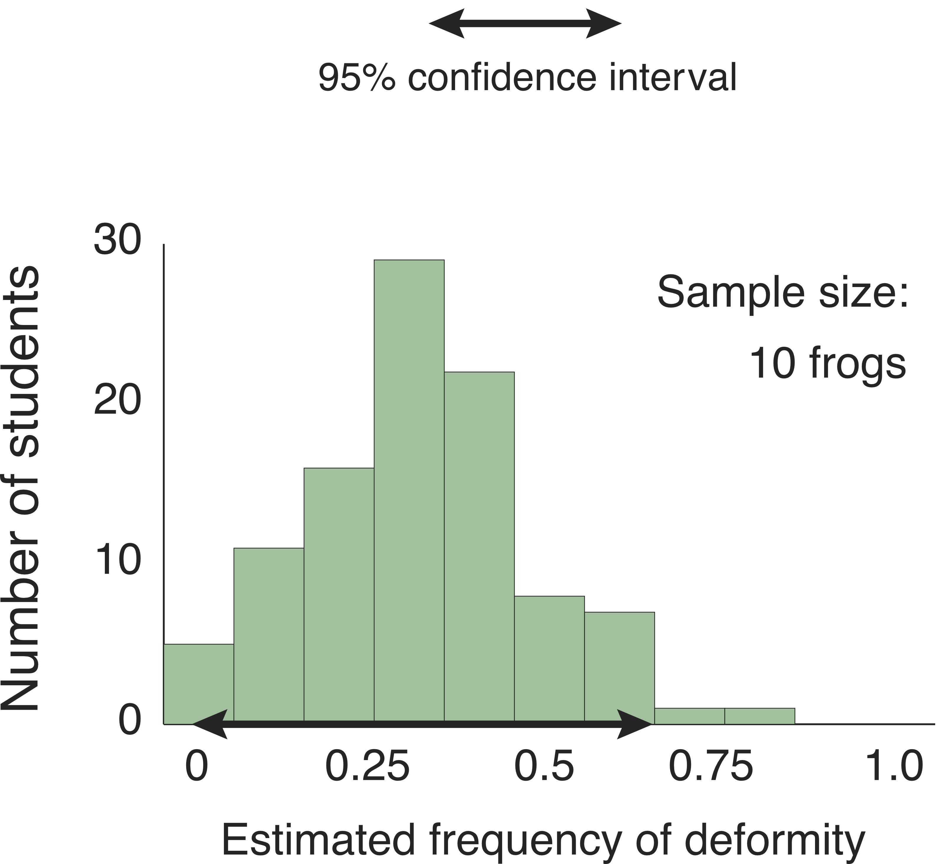
Most of the students’ estimates fall between 20% and 40%. Due to bad luck in picking frogs from the pond, however, a few students got estimates as low as zero or as high as 80%. The double-headed black arrow encompasses 95 of the students’ estimates, excluding only the five most extreme values. Based on the students’ research, they could say with 95% confidence that the true frequency of deformity is between 5% and 70%.

How much better would the students do if they worked twice as hard? To find out, I used the computer to simulate the estimates they would produce if each one caught and examined 20 frogs.

When each of 100 students examined 20 frogs from a population and estimated the frequency of deformity, 95 of their estimates were between 15% and 50%. The true frequency of deformity in the population was 30%.

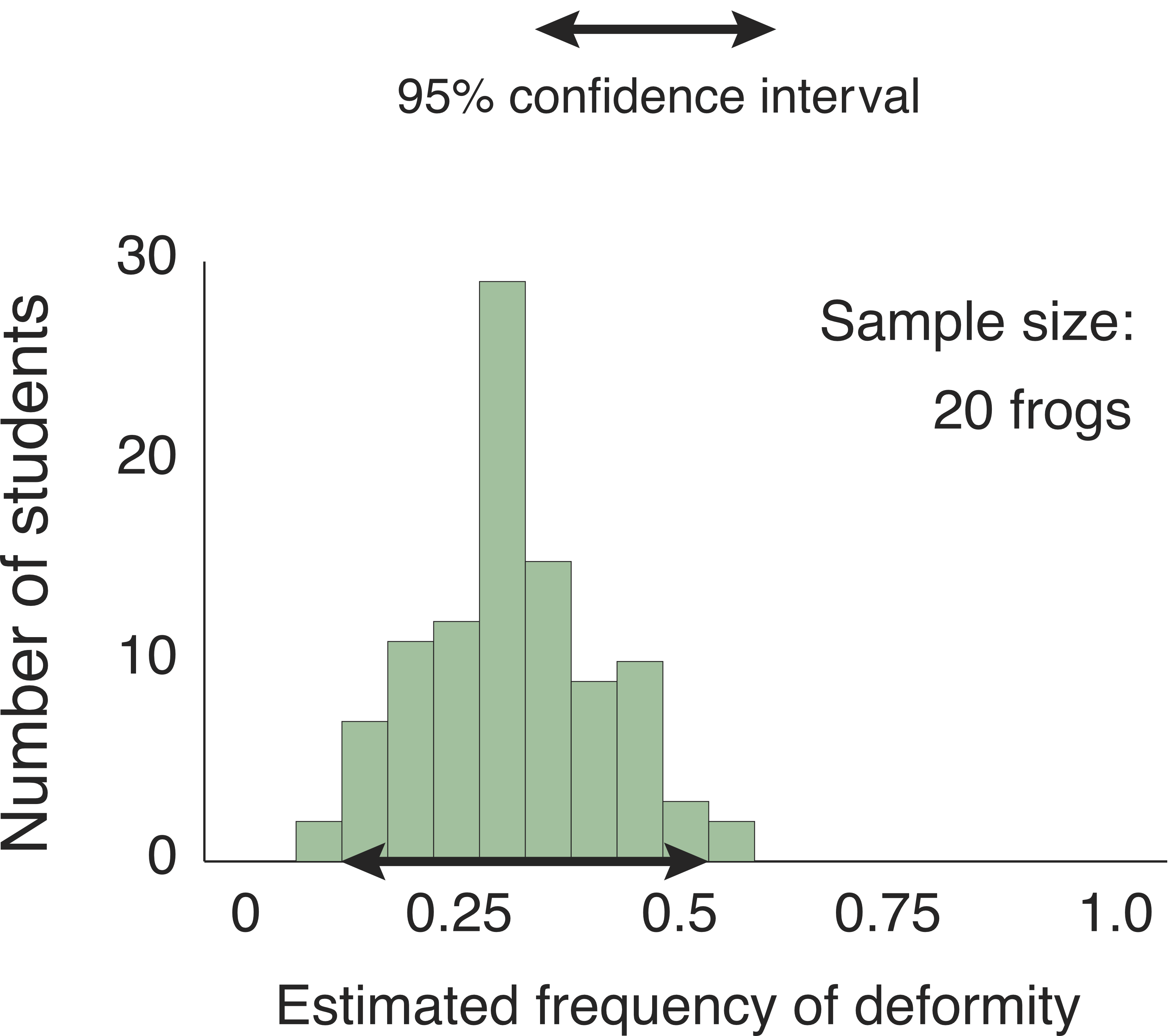
Now the students could say with 95% confidence that the true frequency of deformity is between 15% and 50%.

And if the students worked five times harder still? I simulated the estimates they would produce if each one caught and examined 100 frogs.

When each of 100 students examined 100 frogs from a population and estimated the frequency of deformity, 95 of their estimates were between 19% and 44%. The true frequency of deformity in the population was 30%.

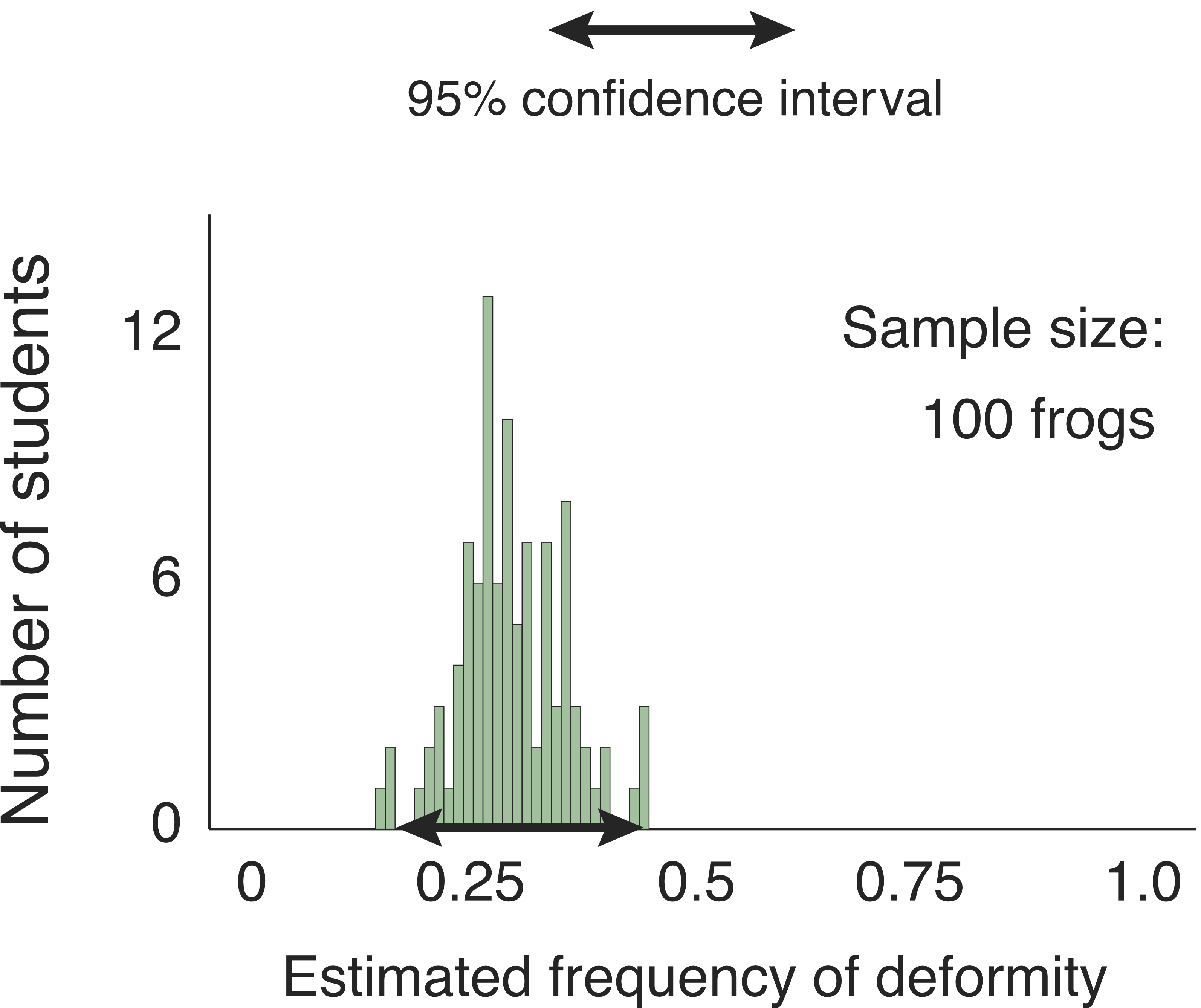
They could say with 95% confidence that the true frequency of deformity is between 19% and 44%

These simulations confirm what intuition already told us: As the students examine more and more frogs, their individual estimates of the rate of deformity cluster ever more closely around the truth.

Now imagine that we are biologists doing a real study of frogs in real pond. We get only one estimate of the rate of deformity, not 100 different estimates. Maybe our estimate is close to the truth, or maybe—due to simple bad luck—it is one of the outliers. We do not know and cannot know which is the case, so we have to allow for the possibility of chance error in drawing conclusions from our study.

A margin of error that is generally considered reasonable is an estimate of the 95% confidence interval. But how can we estimate the 95% confidence interval if we have only one estimate of the rate of deformity? One answer is by pulling up on our own bootstraps. We assume that our estimate of the rate of deformity matches the truth, then use a computer to simulate a large number of repetitions of our study. Some of the simulated studies will produce estimates of the rate of deformity that match our real estimate exactly; some of the simulated studies will show chance errors. The range of values that includes the estimates produced by 95% of the simulated studies will be our 95% confidence interval. If we follow this procedure in every study we do, then our confidence intervals should overlap the truth about 95% of the time.

In the era before computers, statisticians invented, out of necessity, a short-cut approach to calculating confidence intervals. Given the design of a study, the sample size, and the estimated value, we can often use a mathematical formula to estimate the typical size of the chance error we would see in our results if we repeated the study many times. This typical chance error is called the Standard Error, or SE. As an example, imagine that we caught and examined 100 frogs, and found that 30 were deformed and 70 were normal. We can estimate the typical error among replicates of this study as follows:

\[Standard \space Error = \sqrt{100} \space \times \space \sqrt{0.3 \times 0.7} \approx 4.6\]

The 95% confidence interval is given by plus or minus twice the standard error, which in this case is about 9. If we were to repeat the study many times, we could expect that 95% of the time we would find that somewhere between 21 and 39 out of 100 frogs are deformed. We can reasonably say that in the pond we’ve looked at, probably 30±9% of the frogs are deformed.

The most important thing to remember about confidence intervals is that they get smaller with larger sample sizes. This plot shows how the 95% confidence interval of our frog survey would change with the number of frogs we examined (again assuming that the true fraction of deformed frogs is 30%).

The width of the confidence interval decreases with increasing sample size.

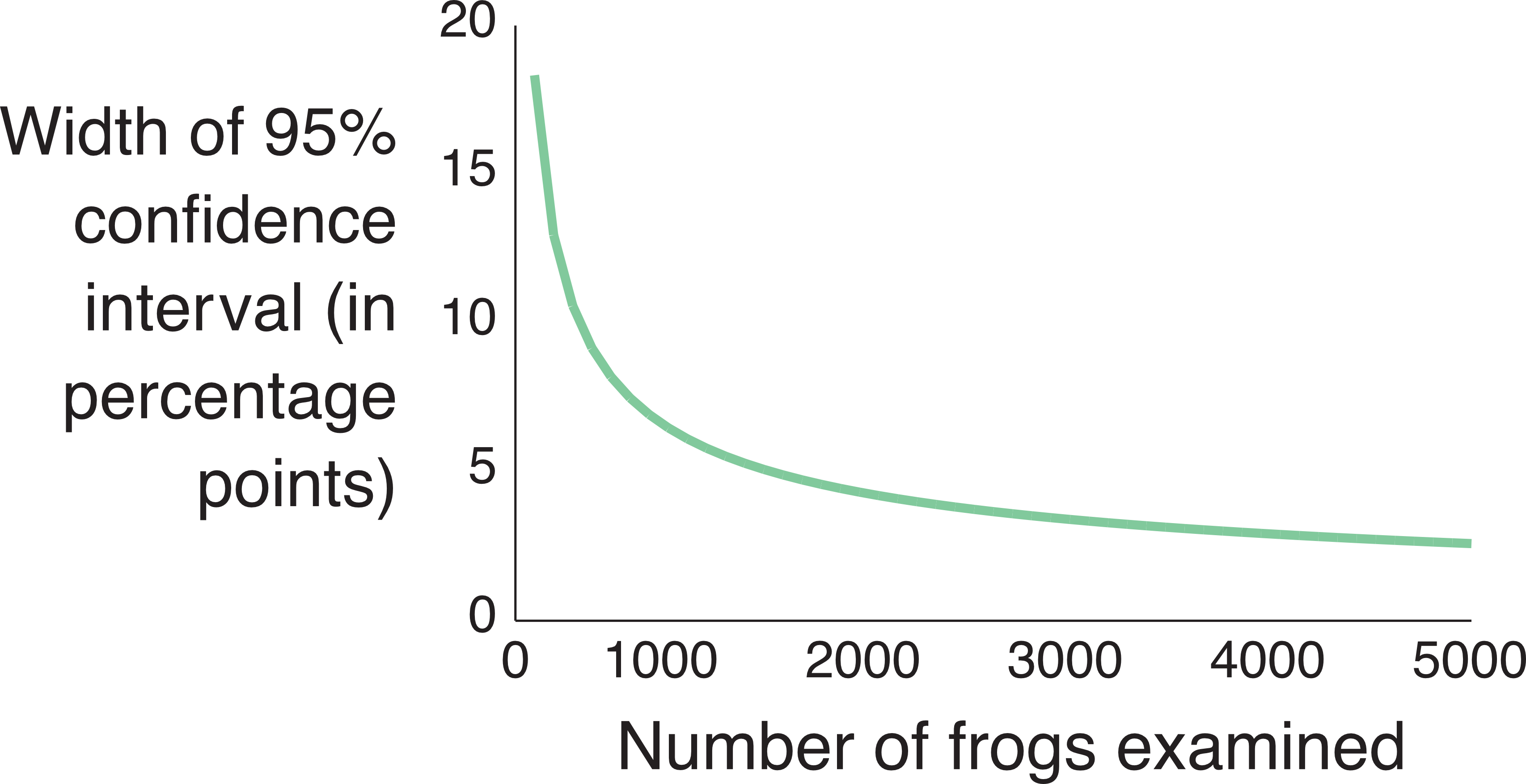
Note that increasing the number of frogs examined from 100 to 1000 gives us a big improvement in accuracy. Increasing our sample size even more continues to improve our accuracy, but rather less dramatically.