Solomon Sea gliders ... later work (Nov 2014-)
Later work, writing the second transport paper
Related pages:
- Some tests and checks
- Overlapping glider missions: Overlaps Example Aviso comparison
- Glider DH sorted by yearday, colored by phi
- Gridding/sampling on phi tests:
Glider DH: DH Demeaned DH
Aviso SLA: SLA Demeaned SLA SLA Bandpass
- Section count by month
- More checks (endpoint selection and etc):
- Check J-index endpoints (v13): Check seasonal fit Seasonal and interannual 5-month running mean
- Check monthly interpolation
- Flight model and D vs K endpoint choices testing:
- Mission by mission: D, K, variable CUM D vs K only
- Fit annual cycle: D, K, variable CUM
- Interannual anomalies: D, K, variable CUM
- Initial checks of Russ's new matlab files (links to TS, and velocity and transport comparisons
- Frequency response diagrams: 151-day triangle 209-day triangle Bandpass
- Glider transport and ENSO indices
- pdfs made for Honiara:
Individual values only
Connected values (2)
5-month triangle (3)
Overlay annual cycle (4)
Yellow-fill anomalies (5)
Add interannual (6)
- Interannual transport and SOI shading (pdf) Glider transport and SOI
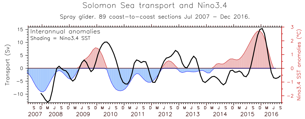
- Interannual transport and Nino3.4 shading (pdf)
- Combined (screenshot of Workplan figure)
- Nino indices 2007-14
- (track,z or sigma) sections for Southern and Northern tracks:
- Track selection maps: Map Show average tracklines
- Crosstrack and salt on z On sigma Add T on sigma
- Checking the endpoint choices RD files)
- Cumulative transport with endpoints marked
- Details near the Sudest/Rossel endpoint (Vectors showing dive numbers and depths)
- Revised 0-700m transport data checking: RD corrected vs BK realtime values.
Use RD values through 135043, then BK values through 146018 (last is 4 Sep 2014).
Adjustments: Omit 2nd sections of 111027 and 11A001, adjust Rossel endpoint of 1st section of 113018. (Notes)
- Mission by mission (Overlay 5-month triangle)
- Annual cycle
- Interannual
- Residual
- Later checks: Transport time series extended through 149043 (Dec 2014)
These made with RD corrected files through 135043 (Aug 2013), then BK realtime files through 149043 (Dec 2014)
- Mission-by-mission values
- 5-month triangle filter Overlay difference
- Layer transports (using RD corrected through 135043, then BK realtime transports through 149043)
- 7 1-sigma layers, 5-month triangle
- Layers grouped above and below sigma 25:
- 5-month triangle
- Annual cycle
- Interannual Overlay TDIR
- Work with latest (sixcharmi) files
Note that the inputs and choices changed a few times. Early plots may be ... wrong?
- Seasonal distribution of samples Dive locations over phi contours
- Various versions of mean/annual cycle vectors on 2 tracks:
- 6 bimonths: v1 Phi by 0.05 Phi by 0.1
- 4 seasons: JFM ... FMA ... MAM ...
- Various (early) uphi explorations:
- Two tracks averaged on phi: Crosstrack vg uphi on z uphi on sigma
- 12 months of uphi (very early)
- Compare sixcharmi with older realtime data: Mission values Annual cycle Interannual (old)
- Interannual:
- Mission values, 3-month RM, annual, interannual
- Interannual transport and Nino3.4 (2014)
- Early comparison: transport, Aviso, Nino3.4
- (Try to) split tracks: values, annual, interannual Overlay combined tracks
- Transport in density layers (old merged data):
- 7 layers
- Above/below sigma 25: 5-month triangle Annual cycle Interannual Overlay TDIR
- Various gridding Uphi(phi,z) on 2 tracks: Dphi=0.1 Dphi=0.05 Separately-gridded tracks
- Add realtime missions 149043 (4), 151001 (4), 153042 (2) (Superseded, see "Work Jan-Feb 2016" below):
- Mission values, overlaid 3-month triangle
- Annual cycle and mean (Compare sixcharmi through 146018)
- Annual-interannual with fill_between
- Overlay Nino3.4
- Looking for fronts
- See earlier work in the "squirts" section on the main SS glider page,
especially "Later exploration of squirts connected to SST fronts"
- Histograms of SST/SSS gradients found in glider data, sorted various ways:
- All (unsorted): SST SSS
- SST histograms sorted by: Time of year SST value Cross-Sea coord. phi
- High SST gradient details for histogram on phi:
- To 0.2°/km Log plot
- To 0.4°C/km: Counts Log of sample fractions
- High-gradient sample locations: Dots for >0.2°C/km Color by mission number Color by magnitude
- Accumulation of high SST gradient in phi-bands (all gradients > 0.1 °C/km)
- 104 largest SST gradients, in phi bands:
Phi=0 to 0.05 (38%) Phi=0.05 to 0.2 (9%) Phi=0.2 to 0.8 (45%) Phi=0.95 to 1 (9%) (None between phi=0.8 to 0.95)
Combined in gradient size order
- Vertical-section and velocity plots to complement the above:
GHR SST, and show on the upper 200m (older version) (new one from sixcharmi files)
- GHR SST year by year, with glider sampling overlaid
(GHRSST and ASCAT winds annual cycle) (GHRSST gradient annual cycle)
- Surface TS diagrams:
Color by phi: All Detail (omit v low S)
Color by month: All Detail (omit v low S)
- Isotherm depth annual cycle on the southern track:
- Measured depths: Z26-Z16 Z16-Z6
- Depth anomalies: Z26-Z16 Z16-Z6
- Annual cycle Z20 and Ekman inference
- Work since Sep 2015
- Transport time series to 158053: Mission-by-mission and 5-month triangle Obs and annual cycle overlay Annual cycle (pdf)
- Interannual and Nino3.4 Transport above sigma 24.5 (pdf)
- Isopycnal depth (all mission overlays):
22.0
22.5
23.0
23.5
24.0
24.5
25.0
25.5
26.0
26.5
27.0
27.2
- Layer transports above isopycnals:
sigma 24
23.0
23.5
24.0
24.5
25.0
25.5
26.0
26.5
27.0
Show correlations with various lags (above sigma 24):
0 months
1 month
2 months
3 month
- Lag correlations of sigma layer transport with Nino3.4
- Layer transports overlaid (unfiltered)
- Experiments separating the two transect directions
- Transect length (days) colored by direction
- Mission-by-mission transport. Dots colored by direction Overlay smooth curve (trantmon)
- Transport differences from the full 5-month triangle: All, dot-color by direction Separate lines for each direction
- Transport comparisons: M-by-M and 5-moth triangle Interannual anomalies
- Annual cycle: Annual cycles from filled time series
But wait: Westbound check Eastbound check Get the wrong answer from the filled data!!!
- Mean uphi and salinity y-anomalies: S contours over uphi The other way around
- Work with the OFES model
- Bottom topography: Solomon Sea
Solomon Islands
Louisiades
Milne Bay
New Caledonia
- Mean vertically-integrated transport vectors: Solomon Sea
Solomon Island region: top-to-bottom
0-1000m
0-300m
- Compare Sol Sea transport to Pacific to its east at 7°S-9°S:
- (x,z) mean sections: Full-depth
0-1200m
Solomon Sea
- Mean x-integral: Full depth
Above 1000m
- Time series
Annual cycle
Interannual
- Define a WBC east of the Solomon chain:
- Mean zint(v)
To 1000m
- Mean v(y,z)
To 1000m
- Seasonal cycle of v(y,z)
- Indonesian Throughflow: Mean indefinite x-integral at several latitudes Interannual transport anomalies
- Work Jan-Feb 2016 (Ocean Sciences prep)
- Sampling distribution plots to 153042 (phi vs t distributions, colored by various things)
- Annual: Year SST Qzav
- Full dates:
Z20: 2007-15 2012-2015 detail
QZAV: 2007-15 2012-2015 detail
- Transport sequence to 15C006: Mission by mission Annual cycle Interannual
- Transport to 15C006 vs Nino3.4
- Layer transport calculations:
- Thickness test plots: Monthly Interannual
- Layer transport test plots: Monthly Interannual
- (t,sigma) contours of transport in layers (interannual)
- Transport summed downwards by layer (all on one page)
- Aviso Solomon Sea zonal-mean vg: All Colored by latitude Overlay glider
Work restarted Jan 2017
- Sol Sea interannual transport and Nino3.4 (through Dec 2016)
- Isotherm depths:
- Mean isotherms and isopycnals (phi,z) Mean isotherm depths (phi,z)
- Isotherm depth stats (phi,T): Amp/phase of annual harmonic RMS of annual and interannual isotherm depths
- Z-isotherm collection, annual and interannual
.