library(ramp.falciparum)
library(deSolve)Superinfection & Queuing
An Introduction to Queuing Theory for Malaria Epidemiology
Complex Infections
A basic question in malaria epidemiology is how long it would take to clear a simple infection. Initial investigations suggested the answer would be counted in months (see the vignette on Infection Duration). Some early studies of malaria exposure counted more than one infecious bite, per person, per day [1]. These sorts of observations gave rise questions about the importance of superinfection, or getting reinfected while infected.1
If people were getting exposed at a higher rate than they were getting infected, then infections become complex – the parasites in blood include parasites from multiple distinct infectious bites. If all the parasites in an infecting bite are called a brood (for lack of a better collective noun), how many broods would be infecting a person? Over the decades, studies of the distribution of the number of broods per person have used the term multiplicity of infection (MoI), a topic we take up in a deep dive elsewhere (see the vignette on the Multiplicity of Infection).
Ross’s model had assumed that infected people would clear parasites at a constant rate, and that they could then become infected again. Given the high rates of exposure, if one parasite clears, a person could still be infected with others. How long would it take before they cleared all their infections?
Walton’s Answer
On the question of the distribution of the MoI, GA Walton gave this answer in 1947 [2]:
Assume that mosquito-bites are distributed at random. Then if \(m\) be the number of infective bites per person per year, the number of person bitten \(0, 1, 2, 3,\) etc. times per year will be in the proportion of the Poisson series: \(e^{-m}(1, m^2/2!, ...)\)
Walton’s answer, at this stage, is framed only in terms of the number of times a person would be infected in a year, but then he goes a bit deeper. Suppose \(q\) is the proportion of those infections that would be detected, then the fraction of people who would test positive is:
\[1-e^{-mq}\] Notably, Walton’s answer involving detection implicitly includes clearance. The formula assumes (correctly) that a Poisson distribution with mean \(m\) that has been compounded with a binomial with probability of detection \(q\) is another Poisson with mean \(mq.\) The fraction who would test negative is the zero term, \(e^{-mq};\) everyone else would test positive.
It would, perhaps, be useful to formulate the underlying mathematics using dynamical systems.
Queueing Theory
While Ross had developed a model for simple infections, that model can be modified to track changes in the MoI. In the modified model, there are as many compartments as needed (potentially infinite), indexed by \(i,\) and the \(i^{th}\) compartment is the fraction of a population infected with \(i\) parasite broods. The MoI increases when infections occur, and the MoI decreases when parasites clear.
Mathematical models that track the MoI were developed to understand queuing: the MoI is like the number of people standing in a queue, waiting to be served. Queuing theory was introduced into malaria epidemiology as an approach to understanding superinfection by Norman Bailey [3].
Queing models are classified by the mathematical assumptions they make about arrivals and departures. In queuing models for malaria, we must make some rigorous assumptions about parasite arrivals and departures:
Exposure and Infection - infections arise through exposure, increasing the MoI. The average rate of increase in the MoI is given by the force of infection (FoI), denoted \(h,\) but different queuing models make very different assumptions about exposure. Exposure could arise in clusters (e.g. Tweedie processes). A single brood includes all the parasites arising from a single bite, but that brood could be complex if the mosquito was superinfected. We probably need a term like clone that is a subset of a brood including all the parasites in a human that trace back to a single genotype just after meiosis in the mosquito.
Clearance - we could assume that parasites clear independently at some exponential rate, \(r,\) but there are many alternative ways modeling clearance in these models. Some alternatives: the parasites might not clear at an exponential rate; clearance might not be independent; and humans could take drugs that clear some or all of the broods;
If we add demographics, the distribution of the MoI in a population is affected by the births and deaths of humans.
Queuing models are classified and named … (Please help, John)
The software in ramp.falciparum includes functions to set up and solve the queuing model \(M/M/\infty\) and some other queuing models.
The following uses a software package called
ramp.falciparum.
M/M/\(\infty\)
We start with the simple assumptions that Walton made: infections arise as a Poisson process, and infections clear independently. The resulting model is called \(M/M/\infty\)
The following diagram shows illustrates how queuing works in the simple queuing model called \(M/M/\infty.\) (The model has it’s own wikipedia page.) The fraction of the population with a given MoI, denoted \(\zeta_i=i,\) changes over time: each time an infection occurs, the MoI increases by one; any parasite could clear, so if the MoI is \(i\) then the fraction of the population declines at the rate \(mi.\)
\[\begin{equation} \begin{array}{ccccccccc} \zeta_0 & {h\atop \longrightarrow} \atop {\longleftarrow \atop r} & \zeta_1 & {h\atop \longrightarrow} \atop {\longleftarrow \atop {2r}} & \zeta_2 & {h \atop \longrightarrow} \atop {\longleftarrow \atop {3r}} & \zeta_3 & {h \atop \longrightarrow} \atop {\longleftarrow \atop {4r}}& \ldots \end{array} \end{equation}\]
The process is described by an infinite system of differential equations. Changes in the fraction uninfected (MoI=0) are described by:
\[\frac{d \zeta_0}{dt} = r \zeta _1 - h \zeta_0.\]
For those who are infected (with MoI\(=i\)), the dynamics are:
\[\frac{d \zeta_i}{dt} = h \zeta_{i-1} + r(i+1) \zeta_{i+1} - (r+h) \zeta_i\] In this system, the distribution of the MoI follows a Poisson distribution.
First, we need a model for the force of infection as a function of age and time:
plot(aa, FoI(aa, foiP3), type = "l",
     xlab = "a - age (in days)", ylab = expression(FoI[tau](a)))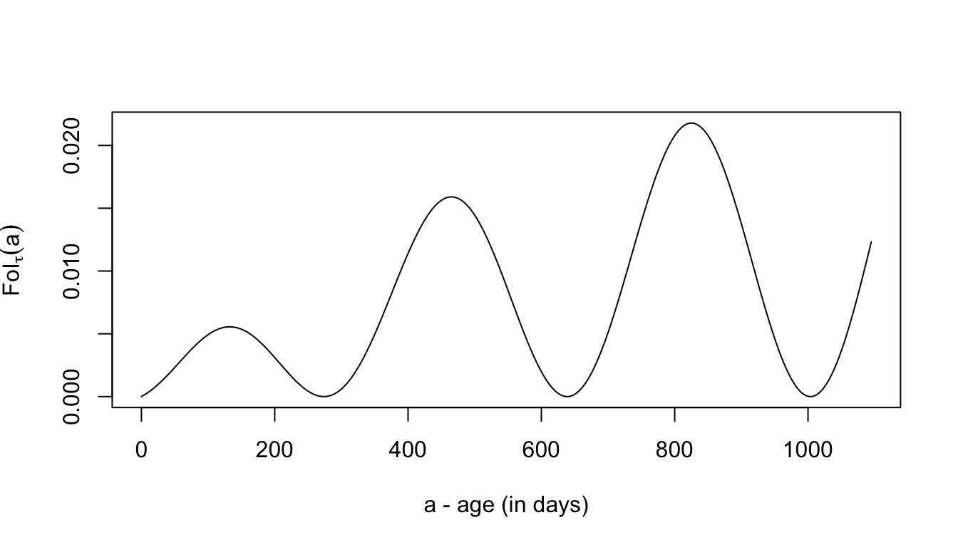
While \(M/M/\infty\) is an infinite system of differential equations, the function solveMMinfinity solves a finite system of differential equations. The maximum MoI is chosen to be large enough that it doesn’t affect the results.
MMinf <- solveMMinfty(5/365, foiP3, Amax=1095)with(MMinf, plot(time, m, type = "l", ylab = expression(m[tau](a)), xlab = "a - cohort age (in days)"))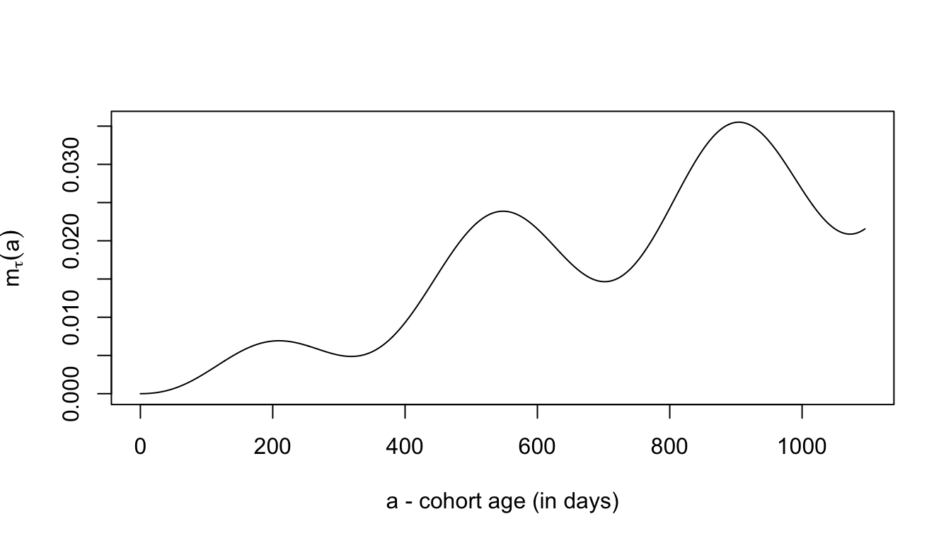
Finite Types
We can consider an alternative model where there are \(N\) types, so if a person is already infected with \(i\) types, there’s a chance that exposure is reinfection with a type the person already has. One sensible assumption is that the MoI increases at the rate \(h(N-i)/N.\)
Write me.
Gamma Exposure
If a mosquito is superinfected, or if we want to model a Tweedie process, then we can assume that infections events arise at the average rate \(h\), but a probability distribution function determines how many infecting clones arise, so a person goes from MoI \(i\rightarrow i+j\) with probability \(P(j)\).
Write me.
Drugs
An alternative model is clearance by drugs.
Write me.
Simple Dynamics
NOTE: In the remainder of this article, we let \(m\) denote the MoI, and we will let \(h\) denote the daily FoI. The notation comes from Ross, who called the FoI the “happenings” rate.
We would like to write down a new formula for the dynamics of malaria with superinfection. In general, we let \(h\) denote the force of infection, and \(r\) the clearance rate, the clearance rate is denoted \(R(h,r),\) and we can write: \[ \frac{dx}{dt} = h (1-x) - R(h,r) x \]
Macdonald & Superinfection
In 1950, George Macdonald published a dynamical model of malaria superinfection [4], where the clearance rate depended on the rate of exposure. In Macdonald’s model, Macdonald describes parasites clearing independently – the same assumptions as Walton – but his mathematical formulas match a different model.
\[
R(h,r) =
\left\{
\begin{array}{rl}
h-r & \mbox{if } h < r \\
0 & \mbox{if } h \geq r \\
\end{array}
\right.
\] Paul Fine’s essay on the problematic formulation of Macdonald’s model for superinfection is highly recommended reading [5].
It’s worth mentioning briefly that Macdonald tended to avoid analysis where the superinfection assumption would have been important. For example, when Macdonald first published his formula for the basic reproductive number, \(R_0,\) the analysis focuses on the dynamics when prevalence is low and superinfection can be ignored [6]. Similarly, when Macdonald led a paper describing the timelines for malaria elimination following the interruption of transmission, he assumed \(h=0\) [7]. In both cases, assumption about clearance ended up being identical to the assumption that Ross made in his simple model (an SIS compartmental model, see The Ross-Macdonald Model).
Garki Approximation
In 1974, Kaus Dietz and collaborators presented slightly different solution to the problem of clearance with superinfection in a mathematical model developed for the Garki Project [8]. In the Garki model, the mean MoI is assumed to be \(h/r.\) The explanation is:
Inoculations “arrive” according to a Poisson process with rate \(h.\) Each inoculation has an exponentially distributed duration with mean \(r^{-1}.\) Then, in inquilibrium, the number of inoculations present at any time is a Poisson variable with mean \(h/r\).
In this model, clearance can only occur if a person is infected with an MoI of one and that infection clears. If the distribution is Poisson with mean \(m = h/r,\) the clearance rate expressed as a function of \(m\) is the probability of having an MoI equal to one, conditioned on being infected at all. Letting \(\zeta\) denote the random variable.: \[
R(m) = r \frac{\mbox{Pr}(\zeta=1 | m)}{\mbox{Pr}(\zeta>0 | m)} = r \frac{m e^{-m}}{1-e^{-m}} = r \frac{m}{e^{-m}-1}
\] Substituting \(m=h/r\)
\[
R(h,r) = \frac{h}{e^{h/r}-1}.
\] The Garki model solution traces is based on a general solution to the problem published in 1957, by Norman Bailey [3]. Bailey had solved used queuing theory, a framework that provides a general way of modeling both superinfection and the distribution. Dietz’s function was based on a steady state solution to a model from queuing theory, called \(M/M/\infty\). In effect, the Garki model assumes that the MoI instantaneously tracks the steady state of a system with the current FoI.
We will deal with queuing theory below, but before we do that, we present a correct solution to Macdonald’s problem.
An Exact Solution
Knowing that the MoI, \(m,\) is the mean of a Poisson, and the prevalence of infection is the complement of the zero term from a Poisson, we get that: \[x = 1 - e^{-m}\] Using \(m,\) the change in prevalence can be described by the equation:
\[ \frac{dx}{dt} = h(1-x)-R(m, r)x \]
We can solve for \(m\), \[m = -\ln(1-x),\] and substitute, such that: \[ R(x, r) = - r \ln (1-x) \frac{(1-x) }{x}\] and noting that \[\lim_{x \rightarrow 0} R(x,r) = r,\] a simple formula for the change in prevalence would be: \[ \frac{dx}{dt} = h(1-x) + r \ln (1-x) \frac{(1-x) }{x} \] This equation is, perhaps, only of academic interest. It involves a strong assumption and a clever trick.
While the equation is correct, it is hiding a lot of complex math. Knowing \(x,\) and knowing the distribution is Poisson, we can always recover \(m.\) Without understanding that math, we’re stuck with this model and the assumption. Since we don’t want to get boxed in, we will want to understand a bit more about how all this works, as well as when the equations would not be appropriate. To do that, we will need to learn a bit about queuing theory. In the following, we formulate some queuing models. We do not know if queuing theory will ever be useful for a malaria analyst, but these ideas are woven through malaria theory, and it is never a bad thing to have an extra tool in the box.
In the next vignette, we present Hybrid Models, we cover some of this math, including an elegant solution to the problem of superinfection developed by Ingmar Nåsell [9].
CAB
The following is a chronological, annotated bibliography (CAB) for superinfection and queuing theory.
1914 – McKendrick’s paper…
1947 – On the control of malaria in Freetown, Sierra Leone; I. Plasmodium falciparum and Anopheles gambiae in relation to malaria occurring in infants. [2]
1950 – The analysis of infection rates in diseases in which superinfection occurs, by George Macdonald [4]
1957 – The Mathematical Theory of Epidemics, by Norman Bailey [3] introduced queuing models as a general way of solving the superinfection problem.
1975 – Superinfection - a problem in formulating a problem, by Paul Fine [5].
References
1.
Davey TH, Gordon RM. The estimation of the density of infective anophelines as a method of calculating the relative risk of inoculation with malaria from different species or in different localities. Ann Trop Med Parasitol. 1933;27: 27–52. doi:10.1080/00034983.1933.11684737
2.
Walton GA. On the control of malaria in Freetown, Sierra Leone; I. Plasmodium falciparum and Anopheles gambiae in relation to malaria occurring in infants. Ann Trop Med Parasitol. 1947;41: 380–407. doi:10.1080/00034983.1947.11685341
3.
Bailey NTJ. The mathematical theory of epidemics. New York: Hafner; 1957.
4.
Macdonald G. The analysis of infection rates in diseases in which superinfection occurs. Trop Dis Bull. 1950;47: 907–915. Available: https://www.ncbi.nlm.nih.gov/pubmed/14798656
5.
Fine PEM. Superinfection - a problem in formulating a problem. Tropical Diseases Bulletin. 1975;75: 475–488.
6.
Macdonald G. The analysis of equilibrium in malaria. Trop Dis Bull. 1952;49: 813–829. Available: https://www.ncbi.nlm.nih.gov/pubmed/12995455
7.
Macdonald G, Goeckel GW. The malaria parasite rate and interruption of transmission. Bull World Health Organ. 1964;31: 365–377. Available: https://www.ncbi.nlm.nih.gov/pubmed/14267746
8.
Dietz K, Molineaux L, Thomas A. A malaria model tested in the African savannah. Bull World Health Organ. 1974;50: 347–357. Available: http://www.ncbi.nlm.nih.gov/entrez/query.fcgi?cmd=Retrieve&db=PubMed&dopt=Citation&list_uids=4613512
9.
Nåsell I. Hybrid Models of Tropical Infections. 1st edition. Berlin: Springer-Verlag; 1985. Available: https://play.google.com/store/books/details?id=o1VZzgEACAAJ
Footnotes
The term superinfection was adopted much later by some mathematical epidemiologists to mean reinfection that displaces an old infection; for example, see Nowak and May (1994) [NowakMA1997SuperinfectionEvolution?].↩︎