eir2pr = function(E, rb=1/400){
   E/(E+rb)
}
E = 10^seq(-1.5,2.8, length.out=100)/365
plot(E*365, eir2pr(E), type = "l", log = "x",  ylab = "Prevalence", xlab = "annual EIR", xaxt="n")
axis(1, 10^(c(-1:2)), c(".1", "1", "10", "100"))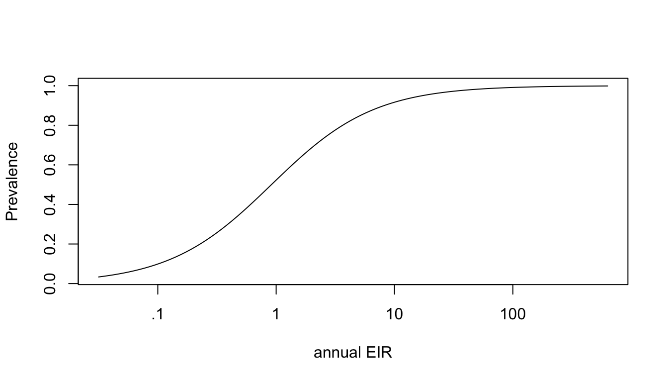
Transmission Intensity, Malaria Metrics, and Outcomes
Simple mathematical models of malaria often get the gist, but when we use them for scenario planning, we are making greater demands of the models. We want to trust the models to make accurate predictions.
Every mathematical model of malaria transmission dynamics and control makes simplifying assumptions. A challenge for malaria analytics is to build models that are up to the task of scenario planning. Given the constraints on available context, this means that models must get scaling relationships right. To illustrate why this matters, we start with the basic model, and we contrast exposure and transmission.
First, we look at the relationship between the EIR and the PR:
\[ dx/dt= b E (1-x)-rx \]
Solving for the steady state, we get:
\[ x = \frac{E}{E+r/b} \]
eir2pr = function(E, rb=1/400){
E/(E+rb)
}
E = 10^seq(-1.5,2.8, length.out=100)/365
plot(E*365, eir2pr(E), type = "l", log = "x", ylab = "Prevalence", xlab = "annual EIR", xaxt="n")
axis(1, 10^(c(-1:2)), c(".1", "1", "10", "100"))
Now we look at transmission. We use Aron’s model, and we get:
\[ E = \frac{M}{H} \frac{fqcx}{g + fqcx} e^{-g\tau} = V \frac{cx}{1+csx} \]
and \(R_0\) is a function of the EIR and the PR: \[R_0 = \frac{bcV}r= E \frac{1+csx}{brx}\]
Now,
\[ x = \frac{R_0-1}{R_0 + c s} \]
In this model, we get a relationship:
ro2pr = function(Ro, cs=1){
  pmax(0, (Ro-1)/(Ro+cs))
}
Ro = 2^seq(-2,3, length.out=100)
plot(Ro, ro2pr(Ro), type = "l", xlab = expression(R[0]), ylab = "PfPR", ylim = c(0,1))
lines(Ro, ro2pr(Ro, .2), lty=2)
segments(3,0,3,1, col = grey(0.5))
All this seems simple enough until we ask the model to make predictions. The main point here is that if all the action in the PR curve occurs for a very small amount of variation in the EIR.
If we try and relate these two curves, we can match values of \(R_0\) and the EIR. Note that for \(R_0 = 8,\) the maximum value in the plot above where PfPR is predicted to be around 80%, the annual EIR is around 3.
ro2eir = function(Ro, cs=1, br=1/400){
  x = pmax(0, (Ro-1)/(Ro+cs))
  Ro*br*x/(1+cs*x)
}
plot(Ro, ro2eir(Ro)*365, type = "l",
     xlab = expression(R[0]), ylab = "PfEIR")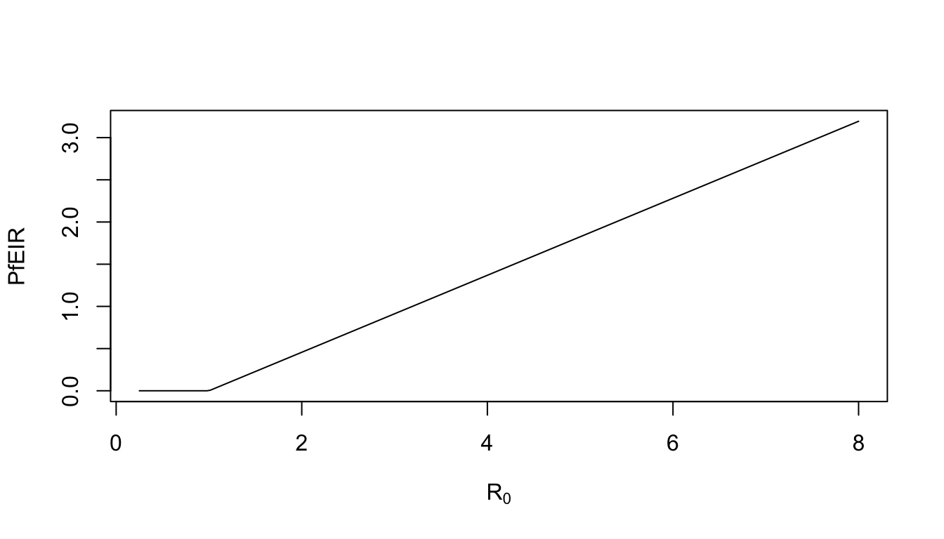
There are three sniff tests that make us suspicious of the quantitative predictions:
In this model, if prevalence is 20%, a 50% reduction in mosquito density would eliminate malaria. If prevalence is around 80%, then an 8-fold reduction in transmission would be enough to eliminate malaria.
The EIR has been estimated at \(~1,500\) bites, per person, per day. In places where the EIR has been estimated in the hundreds, where this model would predict the PfPR ought to be close to 100%. Instead, we find values of the PfPR that are much closer to 30%.
Since the formula for \(R_0\) is inversely proportional to human population density. Human population density varies enormously. Places where human population density is ten times as dense would require ten times as many mosquitoes to get the same prevalence.
The model is wrong in many ways. In real systems:
People take anti-malarial drugs for various reasons, including to treat malaria;
Drug taking varies among population strata;
Exposure varies seasonally;
Exposure is heterogeneous:
there are differences in the expected rate of exposure among population strata; we call this heterogeneous biting
there are differences in the rate of exposure in a population with the same expected rate of exposure; we call this environmental heterogeneity
The model above assumes that all exposure is local, but some malaria is acquired during travel;
The PfEIR varies with age – children get bitten less than adults;
The PfPR varies with age:
Children are born uninfected, but the PfPR rises with age in young children
Beginning in adolescence and extending into adulthood, the PfPR declines with age because of immunity.
Transmission is heterogeneous because of mosquito population structure
All of these factors modify the relationship between the EIR and the PfPR.