Seasonality

Causes and Consequences of Malaria Seasonality

Overview

• Why is malaria seasonal?

• Dynamics with Seasonal Exposure – How does seasonal malaria exposure, a seasonally forced EIR, affect EIR-PR scaling relationships and malaria prevalence?

Seasonal Patterns

This vignette uses SimBA software.

library(ramp.xds)
library(ramp.work)
library(viridisLite)

To develop theory, we want to explore the effects of seasonality on the dynamics of malaria. To do so, we need functions with different seasonal patterns, \(S(t),\) where \[\frac{1}{365}\int_0^{365} S(t) dt = 1\]

This allows us to compare models with the same average annual EIR, denoted \(\bar E.\) Let \(E(t)\) denote the daily EIR at time \(t\): \[E(t) = \bar E \; S(t).\] In effect, \(S(t)\) is giving a weight to days of the year in a way that doesn’t change the mean.

Index of Dispersion

We use the index of dispersion – the variance-to-mean ratio – as a simple way of describing the average dispersion of the seasonal pattern. The index of dispersion of the seasonal pattern is defined as \[ \left(\frac{1}{\bar E}\right)^2 \int_0^{365} \frac{(\bar E - E(t))^2}{365} dt = \int_0^{365} \frac{(1 - S(t))^2}{365} dt \]

compute_iod_S = function(S){
  S2 = function(t, mean){(1-S(t))^2}
  return(integrate(S2, 0, 365, mean=mean)$val/365)
}

compute_iod_S(F_s5)

[1] 0.6443799

compute_iod_F = function(F){
  mean = integrate(F, 0, 365)$val/365
  
  F2 = function(t, mean){(mean-F(t))^2}
  var = integrate(F2, 0, 365, mean=mean)$val/365
  var/mean^2
}

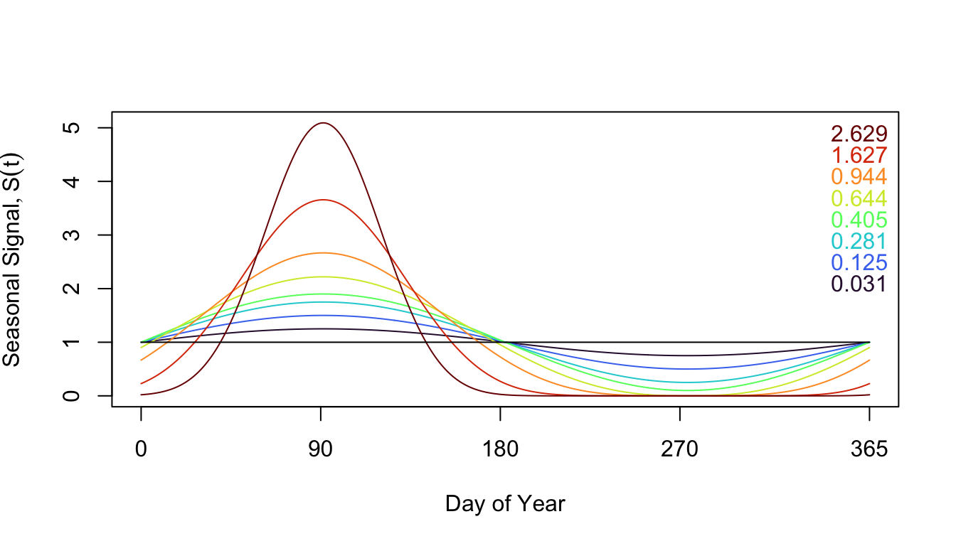
compute_iod_F(F_s5)

[1] 0.6443799

Here, we plot the seasonal signal over a year:

Here we plot 8 different seasonal patterns using sinusoidal functions, and one completely non-seasonal pattern.