Seasonal Exposure

Malaria Dynamics with Seasonal Exposure

---

This vignette uses SimBA software.

library(ramp.xds)
library(ramp.work)
library(viridisLite)

---

Here, we take a general look at malaria seasonality. We begin by asking why malaria is often seasonal, and then we look at some of the consequences of seasonality on the dynamics of malaria.

Seasonal Patterns

We want to explore the effects of seasonality on the dynamics of malaria. To do so, we make a set of functions with different seasonal patterns, \(S(t),\) where \[\frac{1}{365}\int_0^{365} S(t) dt = 1\] For example, if we let \(\bar E\) be the average annual EIR, then the EIR at time \(t,\) denoted \(E(t)\) is: \[E(t) = \bar E \; S(t).\] In effect, \(S(t)\) is giving a weight to days in a way that doesn’t change the mean.

We use the index of dispersion – the variance-to-mean ratio – as a simple way of describing the average dispersion of the seasonal pattern. The index of dispersion of the seasonal pattern is defined as \[ \left(\frac{1}{\bar E}\right)^2 \int_0^{365} \frac{(\bar E - E(t))^2}{365} dt = \int_0^{365} \frac{(1 - S(t))^2}{365} dt \]

compute_iod_S = function(S){
  S2 = function(t, mean){(1-S(t))^2}
  return(integrate(S2, 0, 365, mean=mean)$val/365)
}

compute_iod_S(F_s5)

[1] 0.6443799

compute_iod_F = function(F){
  mean = integrate(F, 0, 365)$val/365
  
  F2 = function(t, mean){(mean-F(t))^2}
  var = integrate(F2, 0, 365, mean=mean)$val/365
  var/mean^2
}

compute_iod_F(F_s5)

[1] 0.6443799

Here, we plot the seasonal signal over a year:

Here we plot 8 different seasonal patterns using sinusoidal functions, and one completely non-seasonal pattern.

Models

NOTE: these models are used by several different projects, so we have made a shared github repository. After running xde_scaling_eir

load("../models/sis.rda")
load("../models/sis_season1.rda")
load("../models/sis_season2.rda")
load("../models/sis_season3.rda")
load("../models/sis_season4.rda")
load("../models/sis_season5.rda")
load("../models/sis_season6.rda")
load("../models/sis_season7.rda")
load("../models/sis_season8.rda")

We now formulate 9 SIS models forced by a seasonal EIR, for each one of the seasonal signals in the figure above.

For each model, we created a mesh of 50 values over \(\log \bar E\) running from 0.1 up to 1000. For each value, the model was run long enough to converge to its stable orbit.

Lags

In the following, we plot PR orbits for different values of \(\bar E\). Note that as \(\bar E\) increases, the timing of the maximum and minimum PR changes relative to the timing of the peak. At low PR, the peak PR trails peak EIR by around 73 days for low EIR. Similarly, trough PR trails peak EIR by about 73 days for low EIR.

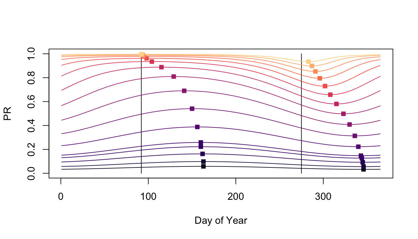
Things look a little different if we increase the strength of the seasonal pattern. In this case, the tro

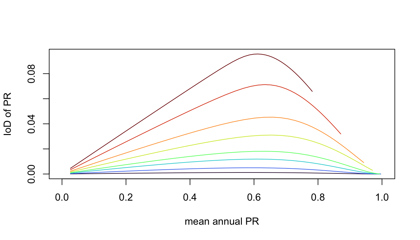
Dispersion of Prevalence

Notice that the index of dipsersion of the PR changes with the index of dispersion of seasonality and with the average annual EIR.

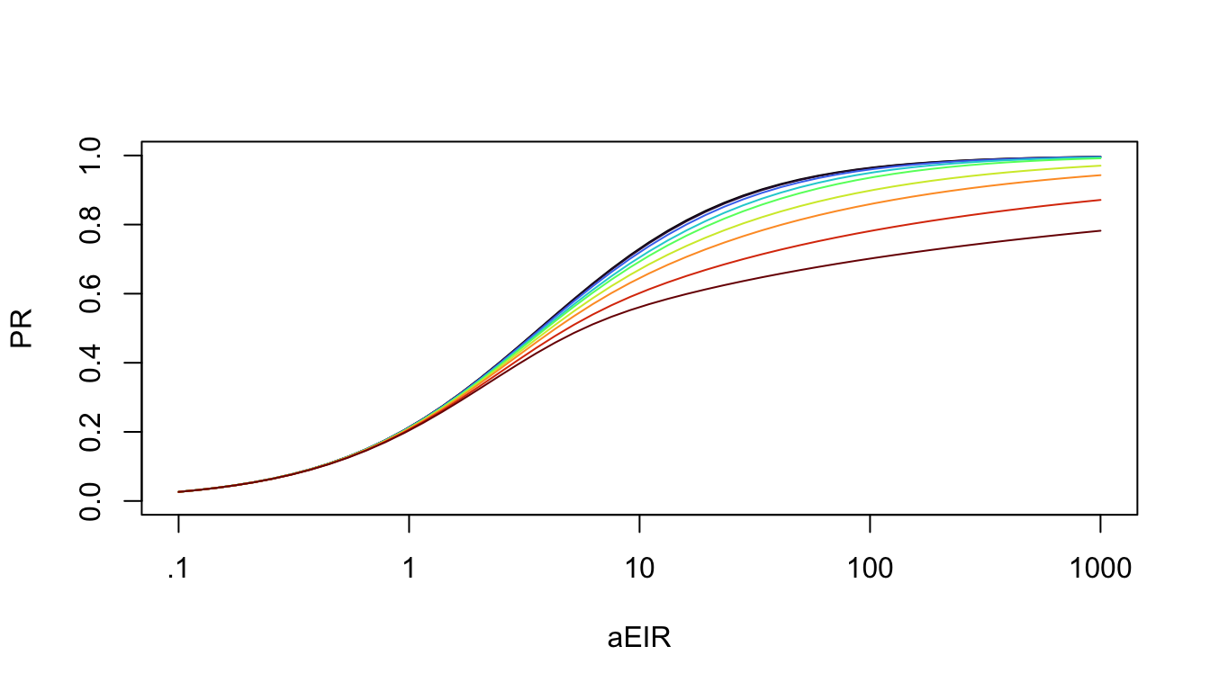
Scaling

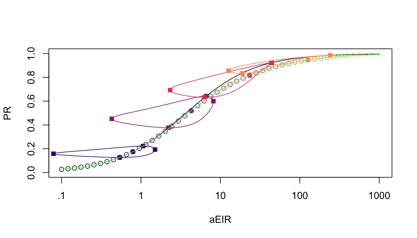
Finally, we can look at the scaling relationships, the average annual EIR versus the average annual PR for all 9 models.

For selected values, we are also plotting the stable orbits.

Note that minimum and maximum PR fall on the line describing the non-seasonal patterns, which is close to the average. if EIR sampling was done at the times of the year when the PR peaked and fell, those values would be on the curve, and likely so would their average.