Ross’s a priori Pathometry
Quantitative Logic for Malaria Dynamics in Populations
A brief, historical introduction the development of mathematical models for malaria in populations.
In 1897, Ronald Ross noticed malaria parasites in the midgut of a mosquito, which was the first direct evidence that malaria parasites were transmitted by mosquitoes [1]. In the years that followed, Ross turned his attention to the Prevention of Malaria [2], when he pioneered the use of mathematics to study malaria in populations [3].
Starting around 1899, Ross’s research was focused on measuring malaria infections and to malaria transmission well enough to make plans for and give advice about malaria control [3]. He was looking for a way of setting rational expectations about the likely outcomes of control. In 1903, for example, he developed the thick film with the goal of improving the accuracy of malaria microscopy [4]. Just as Ross was interested in measuring malaria accurately, he was also interested in understanding why malaria prevalence differed from place to place, and why larval source management had such varied outcomes [5]. Because of the quantitative nature of malaria and the complexity, he used math to organize his thoughts and he developed some of the first quantitative descriptions. He ended up publishing the first mathematical models of malaria: first, a model of mosquito movement [6] and next, two models of malaria transmission [2,7–9].
Quantitative Logic
To develop model for malaria in populations, Ross used a priori quantitative logic – he translated basic ideas about how malaria works in populations into mathematical terms in dynamical systems models – as a complement to statistical analysis. To explain difference in prevalence among populations, he write down equations described infection (through transmission) and the loss of infection in mosquitoes and humans, the processes affecting how malaria prevalence would change over time.
Infection Dynamics
The basic process Ross set out to describe was a model for exposure and infection. Today, we would call it an SIS compartmental model: the population is classified by infection status into one of two compartments – either infected \((I)\) or not infected and susceptible to infection \((S)\), and the total human population is in one of these two states \((H=S+I).\) Rather than present the model as Ross did, we will present it in a rather bare boned fashion.1
Let the variable \(x\) denote the fraction infected, \((x = I/H)\).2
Let the parameter \(h\) denote a hazard rate for exposure, the number of infections, per person, per day; the waiting time to infection is \(1/h\) days.3
Let the parameter \(r\) denote the rate infections clear; the waiting time to clear an infection is \(1/r\) days;
The model assumes that after clearing infections, people become susceptible again. It also assumes that the human population size is constant, so we only really need one equation. As an SIS model, dynamics would be described by:
\[\frac{dI}{dt} = h S - r I = h(H-I)-rI.\] Sometimes, we will see the redundant equation \(dS/dt = - dI/dt.\)
With a change of variables \((x=I/H)\), we get:
\[\frac{dx}{dt} = h (1-x) - r x\]
A simple formula for prevalence at the steady state, \(\bar x,\) is:
\[\bar x = \frac{h}{h+r}\]
At the steady state, the odds of infection are:
\[ \frac{\bar x}{1- \bar x} = \frac {h}{r}\]
We can solve the equation above. Assuming no one is initially infected, the prevalence of infection increases dynamics with respect to age are the solutions:
\[x(t) = \left(1-e^{-(h+r)t}\right) \frac{h}{h+r}\]
These simple dynamics are at the core of simple malaria models. After substituting age for time (and with some minor notational changes), this model is found in a paper by Pull & Grab (1974) to model the infant conversion rate, where the model looked at infection in a cohort of children as they age [10].
Mosquito-Borne Transmission
Simple malaria models involve infection dynamics in two host populations – humans and mosquitoes – connected by parasite transmission through blood feeding. Malaria transmission works as a system with two populations coupled to one another. The process looks something like the following diagram.
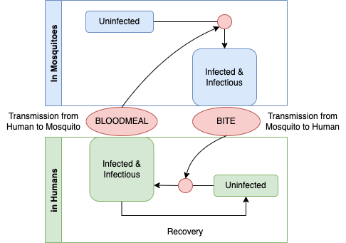
This graph is the basis for causal theory for malaria parasites in populations. A student of causation might object causal graphs must be directed and acyclic, and since this graph is a cycle, it can not be causal. If we applied the logic more generally, no graph describing any organisms life cycle would be causal, and yet life is undoubtedly the cause of life. The missing element is time: a life-cycle graph would be directed and acyclic if it had an arrow that traced life in one generation giving rise to life in the next.
To understand this as a causal diagram, we must thus imagine that it describes a dynamical process in populations: infected mosquitoes today are biting and infecting humans tomorrow; and infectious humans today are causing infections in mosquitoes tomorrow when they take a blood meal. Seen in this way, we can begin to develop a quantitative theory that describes all the factors that determines malaria prevalence in populations. How does malaria persist in a population? It persists through the transmission of parasites among hosts during blood feeding. What factors determine prevalence? It is a balance between the gain and loss of infection.
To write down his model, Ross made some assumptions about the process. We begin with an abstract concept of place – here. We imagine that populations here are comprised of individual mosquitoes and individual humans, and we are interested in computing the fractions of humans and mosquitoes that are infected. Since infections don’t last forever, the prevalence of infection in mosquitoes and humans reflects a balance between infections acquired through parasite transmission and the natural loss of infection through parasite clearance or host mortality. In many places, forces affecting the the balance can be changing; mosquito population density fluctuates over time, for example. Ross’s equations assumed that transmission by mosquitoes was constant over time, and they focused on local transmission, ignoring exposure elsewhere (e.g. through travel). This model thus ignores many factors that would be important for planning for control. Ross discussed all these factors, but since he was pioneering a new approach, the models were very simple.
Mosquitoes
Mosquitoes lived short lives, so the loss of parasites in mosquitoes would mainly occur through mosquito mortality:
\[\begin{equation} \mbox{MOSQUITOES} \\ \; \\ \left[ \begin{array}{rcl} \mbox{Infected Tomorrow} &=& \mbox{Infected Today} \\ &-&\mbox{Infected: Died}\\ &+&\mbox{Uninfected: Got Infected}\\ \end{array} \right] \end{equation}\]This description of a process ignores the loss of infection in mosquitoes, and changing mosquito population density. It ignores the extrinsic incubation period (EIP), the lag between the point in time when a mosquito gets infected and when it becomes infectious. This basic description of the process does not explicitly address the process that gives rise to uninfected mosquitoes. The mathematical formulation implies, without stating it explicitly, that each dying infected mosquito gets replaced by an uninfected mosquito emerging from an aquatic habitat. Otherwise, the mosquito population would declining over time. Ross was interested in malaria transmission dynamics, so the mosquito ecology was almost invisible. Macdonald would address some of these concerns, but Aron’s & May’s equations in 1982 [11] settled many of these issues.
Humans
Humans live long lives, so parasite loss would mainly occur through natural clearance.
\[\begin{equation} \mbox{HUMANS} \\ \; \\ \left[ \begin{array}{rcl} \mbox{Infected Tomorrow} &=& \mbox{Infected Today} \;\; \\ &-& \mbox{Infected: Cleared Infection}\\ &+& \mbox{Uninfected: Got Infected}\\ \end{array} \right] \end{equation}\]This description of the process thus ignores many aspects of human demography, including births, deaths, and migration. The model also ignores a large number of other factors, including super-infection, the complex time course of an infection, immunity, and treatment with anti-malarial drugs. (In Ross’s day, quinine was expensive and difficult to obtain, but it was sometimes used.) These issues have led to many efforts to write down equations describing malaria infection and immunity (see Malaria Epidemiology)
To describe malaria transmission and factors that determine the prevalence of malaria in human populations over time, we formulate mathematical models as dynamical systems. Ross wrote down a system of equations in 1911 [8]. The equations, using his notation, would take this form: \[ \begin{array}{rl} \frac{dz}{dt} &= k' z' (p-z) + q z\\ \frac{dz'}{dt} &= k z (p'-z') + q' z'\\ \end{array} \] where one set of equations would apply to mosquitoes, and the other to humans. Four decades later, Macdonald would recast these equations as part of an enduring synthesis.
Lotka
Alfred Lotka is better known for his work in human demography, and many mathematical epidemiologists will know his basic models for species competition and predation. We are interested in Lotka because of his work on malaria.
Lotka’s interest in malaria traces back to Ross’s 1911 paper in Nature. In 1912, Lotka published a solution to Ross’s equations in Nature [12]. His interest in malaria dynamics culminated in his definitive five-part analysis of Ross’s equations in 1923 [9,13–16]. Ross can be difficult to read, but Lotka’s papers present both of Ross’s models with great clarity.
Macdonald would certainly have known about Lotka’s work on malaria and demography, which is almost certainly where Macdonald got the idea for \(R_0.\) In the fourth part, in a paper led by Lotka’s colleague Sharpe, Ross’s models were extended to include delays, which set the stage for Macdonald’s models [15].
Macdonald
George Macdonald’s analysis of malaria has played an important role in the study of malaria epidemiology and transmission. Curiously, he never wrote down a model for malaria transmission dynamics as a system of differential equations. So what exactly did Macdonald do?
In 1950, George Macdonald published a pair of papers about malaria epidemiology [17,18]. The first paper was a synthetic review of malaria epidemiology, and it included an estimate of the duration of an untreated infection. The second paper presented a new mathematical model for superinfection, but that model had a problem, so it has not been used (see [19]). In 1952, George Macdonald published another pair of papers. In The analysis of the sporozoite rate, Macdonald defined a set of parameters describing malaria transmission and a formula for the sporozoite rate [20]. Macdonald promised that his colleague Armitage would publish a paper to fill in some of the mathematical details. Armitage’s paper, A note on the epidemiology of malaria would appear in 1953, giving mathematical derivations for the superinfection model and the sporozoite rate [21].
Macdonald’s version added an equation – one for the dynamics of infected mosquitoes, and another for the delayed dynamics of infectious mosquitoes – and the parameter values were based on decades of work in malaria epidemiology and medical entomology after Ross (see The Ross-Macdonald Model vignette):
\[\begin{array}{rl} \frac{dx}{dt} &= mabz (1-x) - r x\\ \frac{dy}{dt} &= acx (1-y) - g y\\ \frac{dz}{dt} &= acx_\tau e^{-g\tau} (1-y_\tau) - g z\\ \end{array}\]Macdonald’s analysis of the formula for the sporozoite rate (\(z\), in these equations) demonstrated that transmission was highly sensitive to the mosquito mortality rate.
In The analysis of equilibrium in malaria, Macdonald presented a formula for the basic reproduction rate of malaria parasites, now often called \(R_0\) (pronounced R-naught) [22].
References
Footnotes
We assume a basic familiarity with dynamical systems, mathematical epidemiology, and mathematical ecology.↩︎
The SIS model would typically be presented with equations describing both \(dS/dt\) and \(dI/dt,\) we assume the population size is constant, so one of those equations is redundant. This formula for \(dx/dt\) can be derived from \(dI/dt\) through a change in variables.↩︎
In SIS models for directly transmitted pathogens, we would write \(h = \beta SI\), but here \(h\) involves exposure through blood feeding. To get started, we simply take it as a parameter.↩︎