Glider work around New Caledonia

• SPRAY glider

  (July 17 2005 deployment off the coast of Guadalcanal at 160.14°E,9.47°S):

  A collaboration among      

• Link to Spray #1 home page (Scripps)

• DRAFT   Poster for AGU Ocean Sciences (Honolulu Feb 2006)  version b (650 Mb pdf file)

• Spray #1 at the surface off Bourail, New Caledonia, waiting for pickup (650 Mb jpg photograph)

• (Scanned) article from Les Nouvelles Caledoniennes, Noumea, with photos of us putting the glider in the water for testing in the lagoon (4 July 2005)
  jpg 295Kb   pdf 1.8Mb

Second mission results (Oct 13 2006 deployment off the coast of Guadalcanal at 160.22°E,9.94°S):

1. Page for prep work (maps and historical ADCP data)
2. On-the-fly quick-look plots of raw data:
   1. Map of latest position
   2. Dive-by-dive vectors of vertically-averaged velocity
   3. Along-track sections: Temperature   Salinity
   4. Text list showing latest instrument diagnostics
3. Comparisons between the two missions
   1. Vector velocity   Velocity components
   2. Accumulated transport
4. Mission 2 approaching pickup outside Passe de Yande (1 Mar 07)
5. Some checks, etc
   1. Mission summary plot for Gerard
   2. Trajectory
   3. Salinity along track   T/S near dive 314

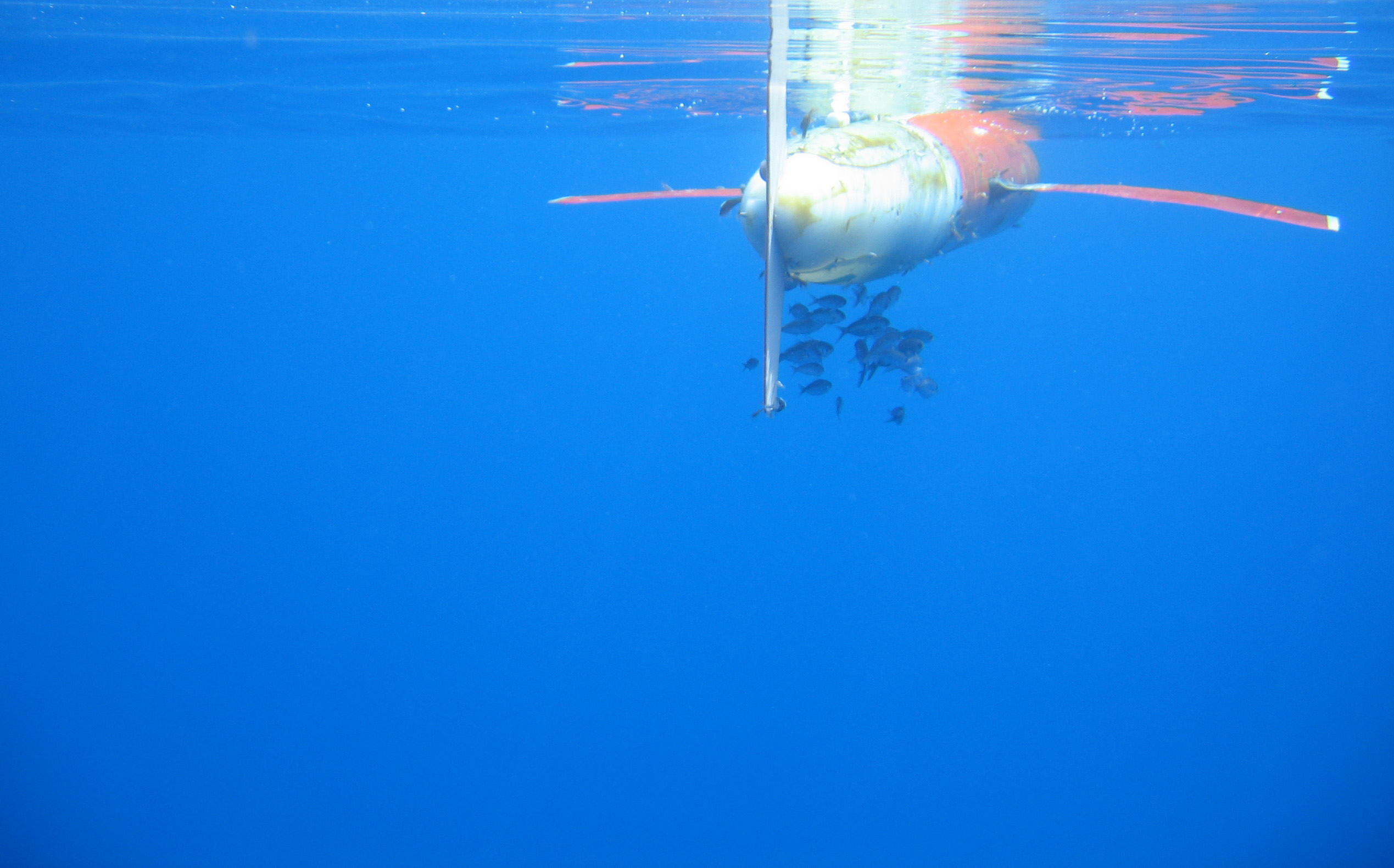
First mission results (July 17 2005 deployment off the coast of Guadalcanal at 160.14°E,9.47°S):

1. Bathymetry and maps
   1. Bathymetry around New Caledonia
      Bathymetry from the Solomons to New Caledonia
   2. Glider distances from NC to Vanuatu and the Solomons
   3. Waypoints near the tip of NC
2. T and S sections
   1. Whole section: T   S   Combined (with map)   (Overlay vectors)
   2. Overlays: S overlay T   Sigma overlay T
   3. TS relation with latitude
   4. Glider S on sigma-25 and S-max
   5. Details near 16°S
      1. T    S    S overlay Sigma    S overlay T
      2. T-S relation
      3. T,S,Sigma profiles from individual dives near 16°S (28 plots)
   6. Combined sections including Secalis3 CTDs (to 2000m): T   S
3. Comparison with CARS climatology and Secalis3 cruise CTDs
   1. Sections: 
      1. Salinity: S on the track   Difference
      2. Temperature: T on the track   Difference
   2. Compare glider S with CARS, Secalis3 CTDs, and Argo (on isotherms):
      1. Glider cruise track with other data sources overlaid
         Bottom depth: Bottom depths at Secalis3 profile locations   Stations and tracks over map
         (See TS plots below for dates)
      2. T and S At 600m: Time series   Scaled difference
      3. S on T=10°C: Time series and difference
      4. S on T=15°C: Time series and difference
      5. All isotherms and mean differences (19 plots)
   3. TS comparisons with Secalis3 cruise CTDs (and CARS climatology and Argo)
      1. TS diagrams (groups of 4 CTD stations): Southern 4   Middle 4   Northern 4   
      2. TS properties spanning the northern reef
   4. Secalis3 CTD sections: Temperature   Salinity   Sigmatheta
   5. Spatial scales (plots of high-pass temperature): North end   South end
4. CARS flow on sigma-25 (Understanding the pattern of high salinity in the thermocline):
   1. Depth of sigma-25   CARS S on sigma 25 and S-max
   2. CARS and ORCA
   3. Streamlines and quantities on sigma-25:
      1. Streamlines and velocity   (Blank where sigma-25 is less than 100m deep)
      2. Velocity over salinity: Vectors   Streamlines
5. Measured currents
   And associated calculations .....
   1. Whole section
   2. Detail of NCJ
   3. Detail of W coast of NC
   4. Glider motion and current components: Dead reckoning    Actual motion    Current speed   
      What if the D.R. speed were 1.1 times as large?   (0.9 times)
   5. u_g from Secalis3 CTDs: u_g section   (plot S to N)
      Compare Secalis3 u_g rel 2000m to glider absolute geostrophy: At 600m   Surface
      Vertically integrated transport from Secalis3 and glider   (Overlay glider u_g)
      Secalis3 Int(u_g)dz (NCJ as a fn of z)
      (Also see Fig.2 in section "Revising the paper" below)
   6. Running integral of transport (and comparisons to other data sets):
      1. Glider
      2. Glider and Secalis3 (u amd u_g rel different levels)
      3. CARS U_g (compare 600m reference levels)   Meridional section of ug(y,z)
      4. Glider. CARS and Island Rule transport   Add Ekman transport   Add Secalis3   Add glider u_g rel 600m
         More recent versions: Filtered   Overlay zonal component   Cut off at 18°S
      5. Ekman transport checks:
         1. Quikscat winds during Jul-Aug 2005   Anomalies   Curl anomalies
         2. Tau and Curl anomalies for Jan-Aug 2005
         3. Ekman transport   In Sv/degree   Vertically-averaged current (compare abs geostrophy)
         4. Ekman transport running integral   Total and seasonal anomalies
      6. CARS 1 cpy annual cycle (note 2 cpy data is flawed, but may be large)
         1. Transport annual cycle
         2. Running integral   Anomalies
      7. Secalis3 CTD running transport integral   
   7. Glider u_g calculation steps and documentation:
      1. Isopycnal depths
      2. Along-track gradient   On sigma
      3. u_g of z
      4. How should sigmatheta be smoothed to compute DH and u_g?
         1. Compare DH with various smoothing: DH   Transport function
         2. Resulting transport   Detail
      5. Glider u_g and measured currents (0-600m average)
      6. Slope of glider track
   8. L-ADCP results (Secalis3):
      1. Lowered ADCP velocity components at 17.55°S
      2. L-ADCP on the east side of the reef: Components   Vectors
      3. Mean L-ADCP velocity on map
      4. L-ADCP vectors in the NCJ core (17.55°S) (Figure for paper)
      5. Compare Secalis3 u_g in the NCJ core   Overlay ADCP at 17.55°S
   9. Absolute cross-track geostrophic velocity   (pdf version; incl both curves)
   10. Velocity estimates from Topex/Jason altimeter
       Interannual anomalies:
       1. Sea level along the glider track
       2. Surface u_g along the glider track   (Check zonal structure of SEC anomalies)
       3. 10°S-20°S average u_g along the glider track
          Annual cycle:
       4. Time series of Topex and CARS sfc u_g, plus CARS transport
       5. 1 cpy harmonic
   11. Glider velocity over altimeter absolute DH: 23 Jul-10 Aug   13-31 Aug
   12. Glider and CARS sigmatheta at 600m
   13. Comparisons with ORCA model:
       1. ORCA mean currents (overlay u)   (overlay glider track)
       2. SEC annual cycle on the glider track
          Jul-Sep mean vs annual mean (sampled along the glider track)
       3. Transport anomalies   Running integral
       4. ORCA sections of u along glider track during JAS: (y,z) section   Surface and 600m velocity

6. Tidal filtering a la Russ:
   1. Filter description (pdf)   Russ's example (Integrated DH)   Difference from Russ's version)
   2. Checks:
      1. Temperature at 600m (first 120 dives): T(t)   (T(y)   Compare original data   Compare 13-pt triangle filter
      2. u_g first 120 dives
      3. Absolute geostrophy: Tide filter (pdf)   Original (spz31 filter) (pdf)
      4. Filter absolute current vectors

1. CARS comparisons: Zonal transport along the track   0-600m only
2. Velocity at 17.55°S:
   1. Secalis3 NCJ velocity   
   2. LADCP: (Revised May 07)   (Original)   Compare: Vectors   Components
   3. Overlay ug and LADCP (revised)   (Original)
3. NCJ transport as a function of ref level (i.e., the transport if the reference level was chosen at depths on the ordinate)
   Compare ug rel 2000m, show results for relevant levels   Simpler (half only)
4. AAIW and water mass checks (Secalis3):
   1. ug as a function of density
   2. Salinity on density:
      1. Overall   Overlay ug
      2. Detail below sigmatheta 26: Overall   Overlay ug
      3. ug and S on 27.2
   3. ug, overlay S
5. Measured current at the coast of Guadalcanal
6. Fig.3 with Island Rule profile (pdf)

Other relevant pages