2. Energy and the First Law

2.1. First Law

The first law of thermodynamics is, in part, a statement of conservation of energy. Although the basic idea of conservation of energy seems intuitive to many readers at present, it took the work of many scientists over a century to conceive and validate before it became a pillar of the modern scientific framework. Beyond conservation of energy, though, there there are subtler and important aspects of the first law that take a little time to unpack.

First, here is a simple mathematical statement of the first law.

(2.1)\[\Delta U = q + w\]

It states that the change in internal energy of a system, \(\Delta U\), is equal to the sum of the heat transferred to the system, \(q\), and the work done on the system, \(w\). Note the following sign conventions that we will use for heat and work. Positive work or heat means that the energy of the system increases, where heat is added to the system or work is done on the system. Most often we will refer to pressure-volume work, where the definition \(w = -\int{P_\textrm{ext}dV}\) from Eq. (1.2) indicates that work is positive for compression of a system and negative for expansion.

Now, beyond conservation of energy, the first law also states that internal energy, \(U\), is a state function despite the fact that heat \(q\) and work \(w\) are path functions. Let’s take a closer look at path and state functions to see why this is both interesting and important.

2.1.1. State and path functions

Imagine hiking a mountain with many routes from the base to the peak (Fig. 2.1). All routes would result in the same change in altitude whereas the distance walked along the specific route could vary considerably from one route to the next. The first law tells us that internal energy \(U\) is a state function–like altitude in the hiking analogy–and that \(\Delta U\) does not depend on the path taken from the initial to final state of the system. This aspect of the first law is intriguing because, somehow, heat \(q\) and work \(w\) are both path functions.

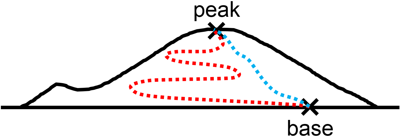
Fig. 2.1 Hiking analogy for path and state functions. The change in altitude between base and peak does not depend on the route taken, and is an example of a state function. In contrast, the distance walked (e.g., red vs blue dashed lines) in general depends on the route and is therefore a path function.

How do we know that work is a path function? Consider the example shown in Fig. 2.2 where a system is taken from point A to point B using the two paths shown in red and blue. Since pressure-volume work is defined as \(w = -\int{P_\textrm{ext}dV}\), with no work being done during the constant volume steps (vertical lines), we can simply judge the work as the area under each path. In that case, the work is larger for the red path than the blue. We could quantify the amount of work in each case. Doing so, we get \(w_\textrm{red}=-P_2\Delta V\) and \(w_\textrm{blue}=-P_1\Delta V\), which for \(P_2>P_1\) and \(\Delta_V\) being negative means that \(w_\textrm{red}>w_\textrm{blue}\). One could even envision a third path where no work is done in which the pressure is first lowered to zero (such as for an ideal gas with temperature approaching absolute zero), the volume is decreased to the final volume, and then the pressure is raised to the final pressure.

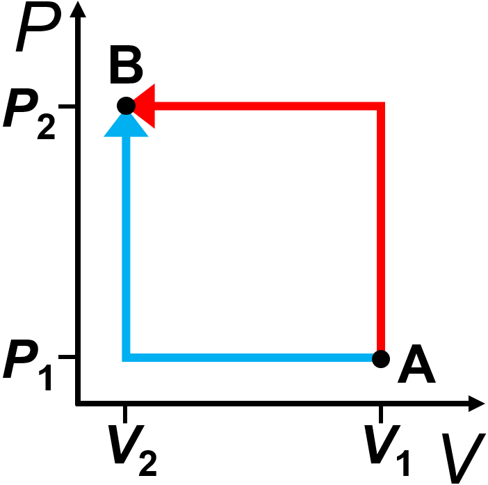
Fig. 2.2 Illustration that pressure-volume work is a path function. Work is the area under each path, where the red path havs a larger magnitude of work done than the blue path.

Sometimes students ask why work is not done during the vertical steps. This can be seen from the definition of pressure-volume work, \(w = -\int{P_\textrm{ext}dV}\), where constant volume leads to \(dV=0\) and therefore \(w=0\). It is also instructive to look at what is happening during those vertical steps, though. For the sake of simplicity, let’s consider that the system being studied is an ideal gas. In that case, if volume is constant but pressure is changing, it must be the case that the temperature is also changing. Keep in mind, however, that this temperature change indicates that heat is added to or removed from the system, not that pressure-volume work is done. The temperature is also changing during the horizontal steps where pressure is constant but volume is changing, so both work and heat are nonzero in those steps.

Hopefully it is clear now that pressure-volume work is a path function. Unfortunately, I am not aware of a way to show that heat is in general a path function. However, it must be. The first law states that internal energy is a state function, and we see clearly that work is a path function, so heat must somehow also be a path function whose “pathiness” cancels out the pathiness of work.

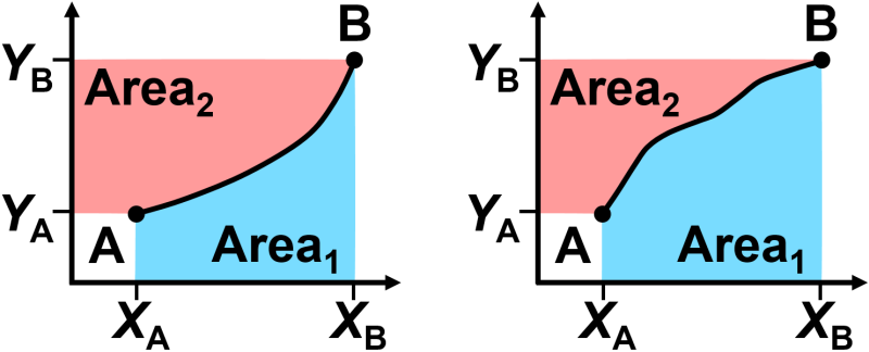
Fig. 2.3 Illustration that two carefully chosen path functions (the pink and blue areas) can add up to a state function (the total colored area). This illustration was adapted from Silbey & Alberty’s text Physical Chemistry [14].

It can be hard to grasp that a state function can be built from the sum of two path functions, so let’s consider a simple visual analogy. In Fig. 2.3, a black curve is shown on each of two x-y plots. We will define \(\textrm{Area}_1\) as the area under the curve and \(\textrm{Area}_2\) as the area to the left of the curve. While \(\textrm{Area}_1\) and \(\textrm{Area}_2\) each depend on the path of the black curve, their sum always adds up to a constant area regardless of the path. Thus the total area is constant regardless of the path, since the path is, after all, just dividing the total area into two different portions. Somehow, this also occurs with the sum of heat and work, even though it is not something we can easily visualize.

\[\begin{split}\textrm{Area}_1 &= \int ydx \\ \textrm{Area}_2 &= \int xdy \\ \textrm{Area}_1 + \textrm{Area}_2 &= \textrm{constant}\end{split}\]

Beyond using state and path functions to better appreciate the deceptive simplicity of the first law, state and path functions are central to other aspects of thermodynamics. In particular, for calculations we will frequently use the property that the change in state functions is identical regardless of the path, as we will see in the upcoming sections. It is therefore useful to have a way to determine whether a function is a state function or not. The Mathematics appendix section on differentials describes a mathematical procedure called Euler’s criterion for exactness for evaluating whether something is a state function or a path function. If you are not already familiar with differentials and Euler’s criterion then you should read that appendix section now.

Test mathematically if total area in Fig. 2.3 is a state function.

Let’s use Euler’s criterion for exactness with the example shown in Fig. 2.3 to see if we can show that the individual areas \(\textrm{Area}_1\) and \(\textrm{Area}_2\) are path functions while the total area is a state function.

\(\textrm{Area}_1\) is defined as

\[A_1 = \int ydx\]

so that its differential is

\[dA_1 = ydx\]

Now, let’s check if the partial derivatives commute. From looking at the differential of \(A_1\) we can see that we already know that

\[\begin{split}\left( \frac{\partial A_1}{\partial x} \right)_y &= y \\ \left( \frac{\partial A_1}{\partial y} \right)_x &= 0\end{split}\]

Then we can take the other partial derivative of each term where we see

\[\left( \frac{\partial}{\partial y} \left( \frac{\partial A_1}{\partial x} \right)_y \right)_x = \left( \frac{\partial}{\partial y} y \right)_x = 1\]

and that

\[\left( \frac{\partial}{\partial x} \left( \frac{\partial A_1}{\partial y} \right)_x \right)_y = 0\]

From this, we can conclude that \(A_1\) is in fact a path function as expected. The same is true for \(A_2\) (try it if you want).

We also expect the total area to be a state function. Let’s see how that plays out with the test for exactness. The total area, \(T=A_1+A_2\), has a differential that is the sum of the differentials for \(A_1\) and \(A_2\)

\[dT = dA_1 + dA_2 = ydx + xdy\]

This time, when looking at the differential of \(T\), we have

\[\begin{split}\left( \frac{\partial T}{\partial x} \right)_y &= y \\ \left( \frac{\partial T}{\partial y} \right)_x &= x\end{split}\]

Now, when we can take the other partial derivative of each term where we see that the outcomes match, showing that the total area \(T\) is in fact a state function.

\[\left( \frac{\partial}{\partial y} \left( \frac{\partial T}{\partial x} \right)_y \right)_x = \left( \frac{\partial}{\partial y} y \right)_x = 1\]

and that

\[\left( \frac{\partial}{\partial x} \left( \frac{\partial T}{\partial y} \right)_x \right)_y = \left( \frac{\partial}{\partial x} x \right)_y = 1\]

2.2. Heat Capacity

The heat capacity is a constant that relates heat added to a system to a temperature change of the system. When the heat capacity is independent of temperature, we can write it as

\[q=n\overline{C}\Delta T \quad \textrm{or} \quad q=mC\Delta T\]

where \(n\) is the number of moles, the molar heat capacity is \(\overline{C}\) in units of J/(K mol), and \(T\) is temperature. The second expression, above, uses mass \(m\) together with the specific heat capacity \(C\) (typically in units of J/(K g)) to generally show the same relationship.

More generally, heat capacity may be temperature-dependent, in which case the heat transferred is the integral of the heat capacity over the temperature range. In the equation, below, the temperature dependence of the heat capacity is stated explicitly using \(\overline{C}(T)\), but whether or not the heat capacity is approximated as being a constant will depend on the specific case.

\[q = \int_{T_1}^{T_2}n\overline{C}(T)dT\]

The differential of the above is \(dq=n\overline{C}dT\). Some texts use a slash through the quantity \(dq\) to emphasize that heat, \(q\), is a path function, but it is a bit cumbersome and doesn’t generally lead to any new insights so we will not use the slash notation.

Since we established above that heat \(q\) is a path function, it may not be surprising that heat capacity is also a path function. That is, the value of the heat capacity will in general depend upon the path taken. Let’s consisder the case of an ideal gas.

2.2.1. Heat Capacity of an Ideal Gas

How much energy does it take to heat \(n\) moles of ideal gas from \(T_1\) to \(T_2\) and why does it depend on whether the volume is fixed or variable?

At constant volume no work can be done on the system. That is, \(w=0\) since \(w = -\int{P_\textrm{ext}dV}\). In that case, the first law becomes \(\Delta U = q\). A (monatomic) ideal gas can only have translational kinetic energy since there are no vibrations or rotations possible with ideal gas particles, and therefore any changes in the kinetic energy of an ideal gas directly relate to changes in the internal energy \(\Delta U\). Fortunately, we already know from the kinetic theory of gases that changes in the kinetic energy of a mole of ideal gas are given by \(n\frac{3}{2}R\Delta T\) so that \(\Delta U = n\frac{3}{2}R\Delta T\). We can put these pieces together to conclude that

\[q=n\frac{3}{2}R\Delta T\]

and therefore the constant volume molar heat capacity \(\overline{C}_V\) is given by

\[\overline{C}_V = \frac{3}{2}R\]

At constant pressure we will obtain a different result. The work term will not be zero since changing the temperature of the gas at constant pressure will result in compression or expansion. Specifically, the work done at constant pressure is \(w=-P\Delta V\), which, when using the ideal gas law, can be converted to \(w=-nR\Delta T\). Now the first law becomes \(\Delta U = q - nR\Delta T\). A sometimes confusing point here is that the change in the internal energy predicted by the kinetic theory of gases depends only on temperature and not on whether or not work is done during the temperature change. Because of this, it is still the case that \(\Delta U = n\frac{3}{2}R\Delta T\). We can put these points together to obtain

\[\Delta U = n\frac{3}{2}R\Delta T = q - nR\Delta T\]

which we can use to solve for \(q\) to obtain

\[q = n\frac{5}{2}R\Delta T_1\]

From this we can see that the constant pressure molar heat capacity \(\overline{C}_P\) is given by

\[\overline{C}_P = \frac{5}{2}R\]

Let’s summarize these two heat capacity results. The heat required to raise the temperature of an ideal gas depends on whether or not the gas can expand. At constant volume, the heat added goes “completely” into increasing the temperature, with a value of \(\overline{C}_V=\frac{3}{2}R\). At constant pressure, the heat added goes into increasing the temperature and to doing work on the surroundings, with a value of \(\overline{C}_P=\frac{5}{2}R\). Therefore it takes more energy to heat a gas at constant pressure than at constant volume. Both heat capacities are temperature-independent for ideal gases, however, real gases have variable heat capacities as we will see shortly.

2.2.2. Heat Capacity of Real Substances

Table 2.1 of measured heat capacities for real gases (values from Wikipedia, with \(T=298 \textrm{K}\)). We can see that for noble, monatomic gases, we are right on the money for \(\overline{C}_V\) and \(\overline{C}_P\)! And for all gases we generally see that \(\overline{C}_P=\overline{C}_V+R\), but \(\overline{C}_V\) seems to depend on the molecule’s geometry. A fuller discussion of why this is the case is out of the scope of a thermodynamics course and requires a little bit of quantum mechanics, so I won’t be covering it in here. What I can say for now is that more complex molecules have more ways to “store” energy than just translational motion, including rotations and vibrations, so when you heat up non-atomic gases, you need to put more energy into the system to get the same temperature increase. The difference between the values of \(\overline{C}_P\) and \(\overline{C}_V\) is relatively constant even for more complicated molecules since it essentially accounts for the amount of work done at constant pressure which approximately obeys an ideal gas even for more more complex molecules.

Table 2.1 Constant pressure and constant volume heat capacities for select gases at ~300 K.

Gas	\(\overline{C}_V\) [J/(K mol)]	\(\overline{C}_P\) [J/(K mol)]
\(\require{mhchem}\ce{CO2}\)	12.5 (1.5R)	20.8 (1.5R)
\(\ce{Ne}\)	12.5 (1.5R)	20.8 (1.5R)
\(\ce{Ar}\)	12.5 (1.5R)	20.8 (1.5R)
\(\ce{H2}\)	20.4 (1.5R)	28.8 (1.5R)
\(\ce{N2}\)	20.8 (1.5R)	29.1 (1.5R)
\(\ce{O2}\)	21.0 (1.5R)	29.4 (1.5R)
\(\ce{CO2}\)	28.5 (1.5R)	36.9 (1.5R)
\(\ce{H2O}\)	28.0 (1.5R)	37.5 (1.5R)

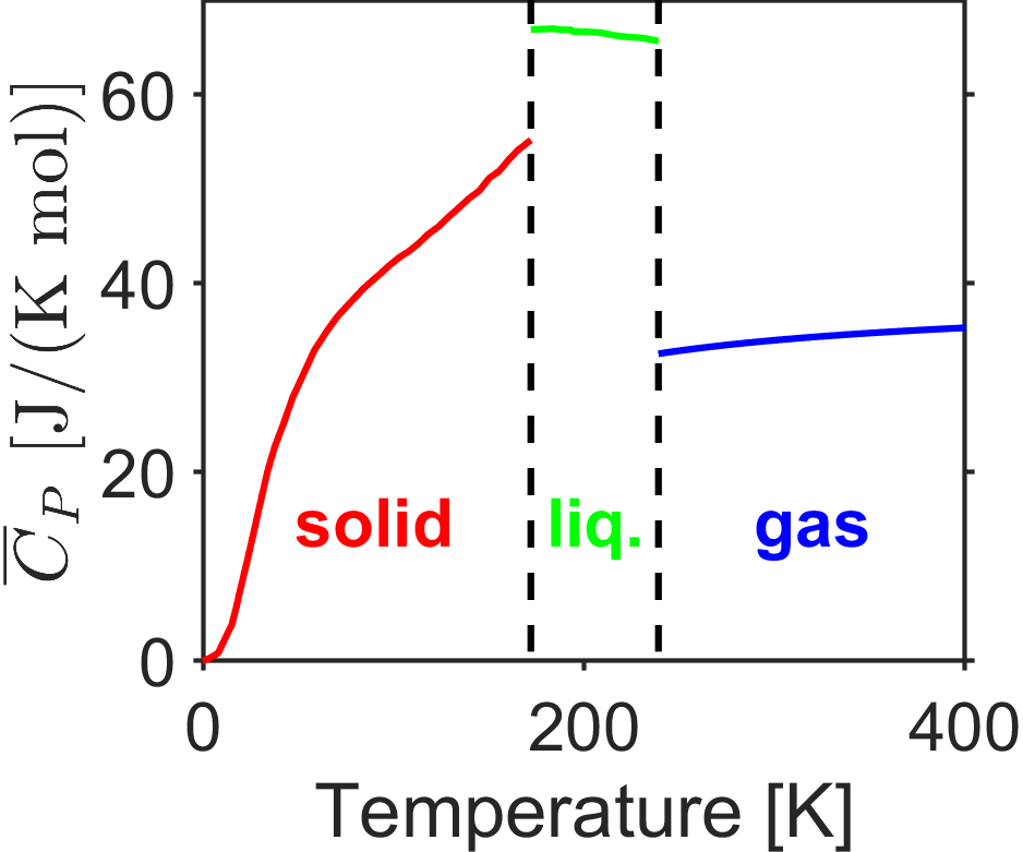
Another important point is that heat capacities change as a function of phase (solid, liquid, gas, etc.) and as a function of temperature. Consider the constant pressure heat capacity data for chlorine in Fig. 2.3 over the range ~0-500 K. The heat capacity is a strong function of temperature for a solid and it approches a value of 0 at absolute zero (more on that when discussing the third law). At phase transitions, the heat capacity jumps abruptly. Furthermore, the heat capacity of the liquid phase is higher than the solid or gas phases due to the substantial intermolecular degrees of freedom; energy must be added to all those intermolecular modes in addition to modes for translation, rotation, vibration, etc.

Fig. 2.4 Constant pressure molar heat capacity for chlorine as a function of temperature. (Data from [15] and [16].) source

2.3. Enthalpy

Although internal energy is a valuable and useful concept, it can be difficult to use. If we wanted to measure heat transferred, we would have to either ensure that experiments are performed in a rigid container so no work is done or we would have to measure the work done in each case. Either would be tedious. Instead, for many experiments or calculations, it would be much easier to work at constant pressure of the system since many of the experiments chemists and biochemists do are at constant pressure. For this reason, we introduce a new energy quantity called enthalpy, symbolized \(H\), which is a convenient measure of energy for constant pressure situations as you will soon see.

Enthalpy is defined as follows.

\[H = U + PV\]

It uses this definition so that the change in enthalpy at constant pressure (of the system) is the same as the heat, or \(\Delta H = q_P\), as shown below. The subscript in \(q_P\) is to indicate heat at constant pressure. Note that enthalpy is a state function since it depends only on other state functions and doesn’t have any integrals, etc., in it.

\[H = U + PV\]

We can use this definition toegether with the first law to see that at constant pressure, \(\Delta H = q_P\).

\[\Delta H = \Delta U + \Delta(PV) = q + w + \Delta(PV)\]

At constant pressure the term \(w=-P\Delta V\) cancels out the term \(\Delta(PV)=P\Delta V\) so that we are left with

\[\Delta H = q_P\]

The basic idea here is that we can change the way we measure energy to best suit our experimental conditions. Mathematically, the definition of enthalpy is a type of Legendre transform. The Gibbs free energy, which we will cover later, is another example of a Legendre transform.

2.3.1. Enthalpy Change for an Ideal Gas

Let’s try to relate enthalpy to heat capacity, now, for an ideal gas. In the calculation, below, note that the ideal gas equation provides that \(\Delta(PV)=nR\Delta T\).

\[\Delta H = \Delta U + \Delta(PV) = n\frac{3}{2}R\Delta T + nR\Delta T = n\frac{5}{2}R\Delta T = n\overline{C}_P\Delta T\]

In the above, recall that we found that the constant pressure heat capacity, \(\overline{C}_P=\frac{5}{2}R\). The relationship \(\Delta H=n\overline{C}_P\Delta T\) is valid for any path, whether constant pressure or not. This is frequently a source of confusion, so let’s take a closer look. Observe that the derivation, above, makes no assumptions about the path. It uses the kinetic theory of gases result that \(\Delta U = n\frac{3}{2}R\Delta T\), which is always true for an ideal gas regardless of path, as well as the definition of work and the ideal gas equation. So, although the constant pressure heat capacity \(\overline(C_P)\) was originally obtained for constant pressure conditions, the equation \(\Delta H=n\overline{C}_P\Delta T\) is always true for an ideal gas regardless of the path. Students in my course often are sometimes confused by the reasoning here, and it is worth taking a little time to think this through before moving on.

Practice ideal gas calculation for changing pressure of the system.

Question: 0.5 moles of ideal gas at 1 atm and 273 K expands against a constant external pressure of 0.1 atm to a final state of 0.2 atm and 210 K. Calculate \(q\), \(w\), \(\Delta U\), and \(\Delta H\).

Answer: Often, some quantities are easier than others to start with for calculations. For an ideal gas, we can determine \(\Delta U\) easily from knowledge of the temperature change.

\[\Delta U = n\frac{3}{2}R\Delta T = 0.5 \textrm{ mol}\frac{3}{2}8.31\frac{\textrm{J}}{\textrm{K mol}}(210 \textrm{ K} - 273 \textrm{ K})= -393 \textrm{ J}\]

For an ideal gas, the change in enthalpy is always proportional to the change in internal energy. Specifically, since \(\Delta U = n\frac{3}{2}R\Delta T\) and \(\Delta H = n\frac{5}{2}R\Delta T\), if you know either \(\Delta U\) or \(\Delta H\) it is straightforward to calculate the other. Note that this does not work with real gases or other substances.

\[\Delta H = \frac{5}{3}\Delta U = \frac{5}{3}(-393 \textrm{ J}) = -654 \textrm{ J}\]

It takes a bit more effort to determine the value of work.

\[\begin{split}w &= -\int P_\textrm{ext}dV = -P_\textrm{ext}\Delta V = -P_\textrm{ext}\left(\frac{nRT_2}{P_2}-\frac{nRT_1}{P_1}\right) \\ &= -P_\textrm{ext}nR\left(\frac{T_2}{P_2}-\frac{T_1}{5P_2}\right) = -\frac{P_\textrm{ext}}{P_2}nR\left(T_2 - \frac{T_1}{5}\right) \\ &=-\frac{0.1}{0.2}0.5 \textrm{ atm }8.31\frac{\textrm{J}}{\textrm{K mol}}\left(210 \textrm{ K} - \frac{273 \textrm{ K}}{5}\right) = -323 \textrm{ J}\end{split}\]

Finally, we can use the first law to get \(q\) as a function of \(\Delta U\) and \(w\).

\[q = \Delta U - w = -392 \textrm{ J} + 323 \textrm{ J} = -70 \textrm{ J}\]

Practice ideal gas calculation for constant pressure of the system.

Question: One mole of ideal gas initially at 300 K and 10 L is compressed at constant pressure to 5 L. Calculate \(q\), \(w\), \(\Delta U\), and \(\Delta H\).

Answer: This time, let’s start by calculating the final temperature from knowledge of pressure, volume, and number of moles. Then we can get \(\Delta U\) and \(\Delta H\) before going on to the other quantities.

\[T_2 = \frac{V_2}{V_1}T_1=\frac{1}{2}300 \textrm{ K}=150 \textrm{ K}\]

so that \(\Delta T = -150 \textrm{ K}\). Next we can get \(\Delta U\) using

\[\Delta U = n\frac{3}{2}R\Delta T = 1 \textrm{ mol}\frac{3}{2}8.31\frac{\textrm{J}}{\textrm{K mol}}(-150 \textrm{ K}) = -1870 \textrm{ J}\]

and, as in the previous worked example we can use \(\Delta H = \frac{5}{3}\Delta U\) to get

\[\Delta H = \frac{5}{3}\Delta U = -3116 \textrm{ J}\]

Since the system is maintained at constant pressure, it must be the case that \(\Delta H = q\) so that

\[q = \Delta H = -3116 \textrm{ J}\]

Finally, from knowledge of \(\Delta U\) and \(q\) we can determine \(w\) using the first law.

\[w = \Delta U - q = -1870 + 3116 \textrm{ J} = 1247 \textrm{ J}\]

It would have also been fine to calculate \(w\) using the work integral as below.

\[\begin{split}w &= -\int PdV = -P\Delta V = -\frac{nRT_1}{V_1}(V_2-V_1)=-nRT_1\left(\frac{V_2}{V_1}-1\right) \\ &= -1 \textrm{ mol }8.31\frac{\textrm{J}}{\textrm{K mol}}300\textrm{ K}\left(\frac{1}{2}-1\right)=1246 \textrm{ J}\end{split}\]

which agrees with the earlier calculation based on the first law.

2.3.2. Enthalpy Change for Phase Transitions

Students learn in elementary school that there are three states of matter including gases, liquids, and solids. These are related to, but should not be confused with, phases. A phase is a distinct form of a substance that is uniform in composition and which is separated from other phases by an interface or phase boundary. Many substances have multiple phases within one state of matter, such as water which can adopt many possible solid phases depending on the temperature and pressure, where each of these phases has a different arrangement of atoms in a crystalline lattice. Or the metal tin can adopt a solid ‘white tin’ phase with a body-centered tetragonal crystal structure and a solid ‘gray tin’ phase with a face-centered diamond-cubic crystal structure.

It is also possible to have a mixture of substances within one phase. Consider a solution of water and acetone, which can be mixed in any proportions and would exist in the liquid phase. If some of the solution were to evaporate into the gas phase above the liquid, then there would be a phase boundary that demarcates the interface between the liquid phase and the gas phase.

When a substances undergoes a phase change such as boiling or freezing, heat may be absorbed or released by the system. This is called the ‘heat of transformation’ or sometimes ‘latent heat’, ‘heat of fusion’, etc., and it may be relatively straightforwardly calculated using tabulated values. Note that such tables typically list only half of the possible phase transitions and that values are generally tabulated as positive; the user must manually insert the correct sign for the enthalpy change. For instance, Table 2.2 lists the enthalpy of fusion (which refers to melting and comes from the latin word fundere) but does not separately list the enthalpy of freezing since it has the same value but opposite sign. Users need to recognize that the enthalpy of fusion appplies to both melting or freezing and need to know to use a positive value for melting (since heat is added when melting) but a negative value for freezing (since heat is lost when freezing). A last note is that the enthalpy changes are tabulated for their corresponding equilibrium phase transition temperatures (with the pressure specified) and the enthalpy changes may be different at other temperatures (see Section 2.5) or pressures (see Section 4.4.2 and Section 4.8.1).

Table 2.2 Select heats of transformation and their equilibrium melting or boiling temperatures at 1 bar (~1 atm).

Substance	\(T_\rm{m} [\rm{K}]\)	\(\Delta H_\rm{fus}^\circ\) [J/mol]	\(T_\rm{b} [\rm{K}]\)	\(\Delta H_\rm{vap}^\circ\) [J/mol]
\(\ce{H2O}\)	273	6,010	373	40,700
\(\ce{EtOH}\)	159	4,973	351	38,560
\(\ce{Hg}\)	234	2,290	630	59,110

For instance, what is the enthalpy change when 3 moles of water freezes at 273 K?

\[\Delta H = - n \Delta H_\textrm{fus} = -3 \textrm{ mol} \times 6010 \textrm{ J/mol} = -18,030 \textrm{ J}.\]

Note that we used the enthalpy of fusion (which is technically melting) for the enthalpy of freezing and inserted a negative sign since we know that the enthalpy change must be negative for freezing since heat is lost by the system.

2.4. Thermochemistry

Thermochemistry is the study of the heat absorbed or released during a chemical reaction or process. It is important for choosing a good fuel to burn, for managing heat loads in batteries, for determining metabolic efficiency, etc. In the kitchen or the lab, we often notice that chemical reactions may lead to a temperature change. Exothermic reactions release heat (\(q<0\)) and tend to heat the sample, while endothermic reactions absorb heat (\(q>0\)) and tend to cool the sample.

Endothermic and Exothermic Reactions…

Question: If an endothermic reaction absorbs heat (\(q>0\)), why does it tend to cool off? Similarly, if an exothermic reaction releases heat (\(q<0\)), why does it tend to heat up?

Answer:

If you remove some heat from some water, for instance, then it is true that its temperature would decrease. Similarly, if you add heat, then the temperature would increase. Sometimes that logic confuses students about the expected temperature change for an endothermic or exothermic reaction. What’s missing?

Remember that heat spontaneously flows from hotter objects to colder ones that are in thermal contact. In the case of a reaction that tends to cool off, heat flows in from the surroundings (\(q>0\)) precisely because the reaction tends to cool off. And if a reaction tends to heat up, heat can flow out to the surroundings (\(q>0\)).

Does that mean endothermic reactions always cool off and do exothermic reactions always heat up? Well, no. If you had a well-mixed reaction that occurs sufficiently slowly and in a container that has a good thermal contact with a constant temperature bath, then the temperature would be constant or very, very close to constant.

A cornerstone of thermochemistry is that enthalpy is a state function. One can consult tables of enthalpies of formation for many compounds and then determine the enthalpy change for a reaction of interest.

2.4.1. Standard State

The standard pressure used for enthalpy of formation of a substance is 1 bar (0.987 atm) and the temperature is typically designated as 298 K. This condition is called standard state and is designated by the little superscript circle such as \(\Delta H^\circ\). For solutions or biochemical reactions there are sometimes additional details for standard state such as using a certain concentration or pH or ‘background’ concentration of ATP or Mg, etc. These conventions are specific to a specific discipline and won’t be a focus here. Lastly, if reactants or products are not at standard state, when doing calculations, it may be necessary to calculate the enthalpy change for converting a non-standard state substance to standard state.

2.4.2. Enthalpy of Formation

Enthalpy, like internal energy, does not have an obvious absolute reference. This is actually a bit of a thorny problem, since the number of possible substances is vast and tabulating the energy changes between all possibilites would be simply impossible. Scientists devised an elegant workaround, however. Since all matter is composed of the same ~100 atomic building blocks, elemental substances are defined to have an enthalpy of formation in their most pure, stable form at standard state. Then, the enthalpy of formation of all possible substances can be tabulated relative to the pure atomic forms.

Be careful as some elements can adopt more than one pure form. For instance oxygen gas \(\ce{O2}\) and ozone gas \(\ce{O3}\) are both composed solely of oxygen atoms but diatomic oxygen, \(\ce{O2}\), is the stabler form and it is defined as having an enthalpy of formation of zero (ozone has a positive enthalpy of formation). Similarly, solid diamond and graphite are both allotropes of carbon, but graphite is stabler in the thermodynamic sense (converting diamond to graphite releases heat) and therefore graphite is defined as having an enthalpy of formation of zero. Similarly, gaseous \(\ce{N2}\), solid magnesium, and liquid mercury all have an enthalpy of formation of zero. A well-known exception is phosphorus; while red and black phosphorus are thermodynamically more stable than white phosphorus, they are much harder to prepare and characterize than white phosphorus.

Once a proper reference system is established, then the enthalpies of formation of substances of interest may be measured by scientists (or sometimes predicted computationally) through the reaction of substances with known enthalpy of formation. The general equation used for these is shown below, where enthalpy of formation is indicated as \(\Delta _fH^\circ=0\), reactants use the index \(i\), and products use the index \(j\).

(2.2)\[\Delta H^\circ_\textrm{rxn} = \sum_i^\textrm{prod} n_i \Delta _f H^\circ_i - \sum_j^\textrm{react} n_j \Delta _f H^\circ_j\]

A scientist would plausibly be able to measure the heat released through the combustion of hydrogen in order to determine the enthalpy change for the reaction.

\[\ce{H2 + 1/2O2->H2O}\]

In this case, since hydrogen and oxygen are already both in their stablest elemental form, then the enthalpy change of the reaction would simply be equal to the enthalpy of formation of water. So, by measuring the heat given off by the combustion of hydrogen with oxygen, the enthalpy of formation of water vapor could be determined as \(\Delta _f H^\circ_{\ce{H2O}}=-242 \textrm{ kJ/mol}\).

Sometimes students get confused by what I call the per mole of what? problem arising from the fact that there are many valid ways to balance a chemical reaction. The reaction of hydrogen with oxygen can in principle be balanced in an infite number of ways.

\[\begin{split}\ce{H2 + 1/2O2 -> H2O} \\ \ce{2H2 + O2 -> 2H2O} \\ \ce{3H2 + 3/2O2 -> 3H2O}\end{split}\]

The first balanced reaction would give an enthlapy of reaction of -242 kJ/mol, while the second give -484 kJ/mol, and both would be correct. This problem may be avoided by stating clearly that the enthalpy change for a reaction is indicated as either per mole of \(\ce{H2}\) or per mole of a specific reaction as written.

2.4.3. Thermochemistry Practice Calculations

Let’s do a few practice problems with enthalpy calculations using Table 2.3, below.

Table 2.3 Select enthalpies of formation at 1 bar (0.987 atm), 298 K.

Substance	\(\Delta_f H^\circ\) [kJ/mol]
\(\ce{H2O}(g)\)	-242
\(\ce{CO2}(g)\)	-394
\(\ce{C2H6O}(g)\)	-235
\(\ce{Al2O3}(s)\)	-1670
\(\ce{C4H10}(g)\)	-126
\(\ce{MgO}(s)\)	-601
\(\ce{Fe2O3}(s)\)	-824
\(\ce{CH4}(g)\)	-75

1. Calculate the enthalpy change for combustion of 2 mole of magnesium by oxygen or carbon dioxide. For this problem, notice first of all that (solid) magnesium and gaseous oxygen both have an enthalpy of formation of zero since they are both elemental substances in their stablest form at 298 K, 1 bar. That is why these substances are not included Table 2.3.

For the combustion of magnesium by oxygen

\[\ce{2Mg(s) + O2(g) -> 2MgO(s)}\]

we can apply Eq. (2.2)

\[\begin{split}\Delta H^\circ_\textrm{rxn} &= 2\Delta_f H^\circ_\textrm{MgO} - 2\Delta_f H^\circ_\textrm{Mg} - \Delta_f H^\circ_{\ce{O2}} \\ &= -1202 \frac{\textrm{kJ}}{\textrm{mol}} -0 -0 = -1202 \frac{\textrm{kJ}}{\textrm{mol}}\end{split}\]

For the combustion of magnesium by carbon dioxide note that carbon (graphite) will be produced, where graphite has an enthalpy of formation of zero,

\[\ce{2Mg(s) + CO2(g) -> 2MgO(s) + C(s)}\]

We can again apply Eq. (2.2)

\[\begin{split}\Delta H^\circ_\textrm{rxn} &= 2\Delta_f H^\circ_\ce{MgO} + \Delta_f H^\circ_\ce{C} - 2\Delta_f H^\circ_\ce{Mg} - \Delta_f H^\circ_{\ce{CO2}} \\ &= -1202 \frac{\textrm{kJ}}{\textrm{mol}} + 0 - 0 + 394 \frac{\textrm{kJ}}{\textrm{mol}} = -808 \frac{\textrm{kJ}}{\textrm{mol}}\end{split}\]

2.5. Alternate Paths

Often we are unable to calculate a quantity directly based on the available information. However, when we are calculating a quantity that is a state function such as \(\Delta U\) or \(\Delta H\) it is perfectly valid to devise an alternate path that connects the initial and final states in order to facilitate the calculation. This idea applies very broadly to thermodynamics and we will return to it many times. Let’s consider the following example of how to do this.

You somehow obtain 1 mol of ‘supercooled’ liquid water at 263 K. What is the enthalpy change upon freezing to solid ice at 263 K? The melting temperature of water is 273 K. The heat capacities of ice and water can be assumed to be independent of temperature here, with \(\overline{C}_\rm{P,liq}=75.4 \rm{\frac{J}{K mol}}\) and \(\overline{C}_\rm{P,sol}=38.1 \rm{\frac{J}{K mol}}\). The enthalpy of fusion at 273 K is \(\Delta H_\rm{fus,273K}=6010\rm{\frac{J}{mol}}\).

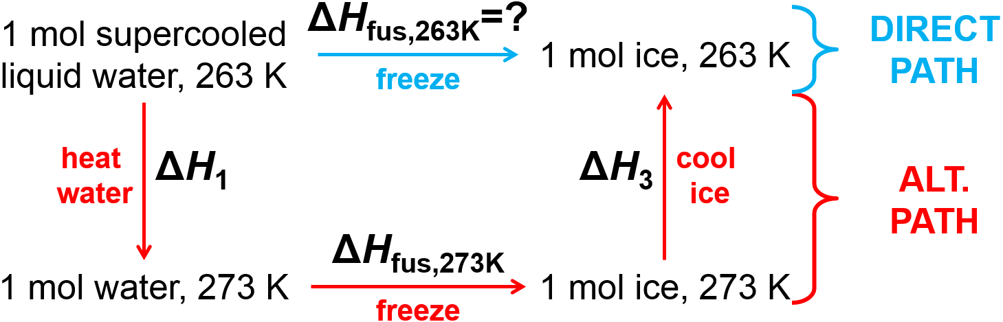
Fig. 2.5 Alternate path enthalpy calculation for freezing of supercooled water.

Since enthalpy is a state function, we can construct whatever path we want between the initial and final states then just calculate the enthalpy change along that alternate path. Fig. 2.5 illustrates the construction of an alternate path that uses the provided information in order to calculate enthalpy changes along three separate steps that connect the desired initial and final states. These can be calculated individually as follows. Note that for this problem, the temperature has been shifted by 10 K from the normal equilibrium freezing temperature of 273 K so we will define \(\Delta T=10\textrm{ K}\) for this calculation since, as you will see, it will come up twice.

Along the alternate path, the enthalpy change for the heating/cooling steps (\(\Delta H_1\) and \(\Delta H_3\)) can be calculated using the provided heat capacity and temperature change and the enthalpy change for freezing at 273 K is provided directly in the problem. Notice that care was taken with the signs here in the alternate path calculation. The temperature change was positive for the heating step and negative in the cooling step, and a negative enthalpy of fusion at 273 K was used in the second step.

\[\begin{split}\Delta H_\rm{fus,263K} &= \Delta H_1 + \Delta H_2 + \Delta H_3 \\ &= n \overline{C}_\textrm{P,liq} \Delta T + n\Delta H_\textrm{fus,273K} + n \overline{C}_\textrm{P,sol}(-\Delta T) \\ &= n(\overline{C}_\textrm{P,liq}-\overline{C}_\textrm{P,sol})\Delta T + n\Delta H_\textrm{fus,273K} \\ &= 1 \textrm{ mol} \times 37.3 \rm{\frac{J}{K mol}}10\textrm{ K} + 1 \textrm{ mol}\times (-6010 \rm{\frac{J}{mol}}) \\ &= -5640 \textrm{ J}\end{split}\]

Practice alternate path enthalpy calculation.

Question: Calculate the enthalpy change at 1 atm for the formation of lactic acid (\(\ce{C3H6O3}\)) from glucose (\(\ce{C6H12O6}\)) at 310 K. The enthalpies of formation at 298 K are \(\Delta_f H_{\textrm{glu,298K}}^\circ=-1274.5 \textrm{ kJ/mol}\) and \(\Delta_f H_{\textrm{lac,298K}}^\circ=-694.0 \textrm{ kJ/mol}\). The molar heat capacities of glucose and lactic acid (assumed to be independent of temperature) are \(\textrm{218.2 J/(K mol)}\) and \(\textrm{127.6 J/(K mol)}\), respectively.

Answer: First, let’s write out a balanced chemical reaction.

\[\ce{C6H12O6->2C3H6O3}\]

Next, let’s figure out the alternate path to be used.

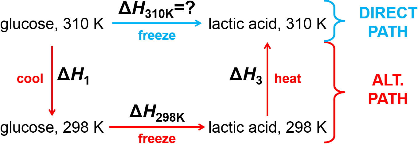
Fig. 2.6 Alternate path for conversion of glucose to lactose.

Now, let’s do the math, where the temeprature difference is defined as \(\Delta T = \textrm{12 K}\). This will be written out per mole of the chemical reaction as written, above.

\[\begin{split}\Delta H_{\textrm{298K}} &= 2\Delta_f H_{\textrm{298K,lac}}^\circ - \Delta_f H_{\textrm{298K,glu}}^\circ \\ &= 2\left(-694 \frac{\textrm{kJ}}{\textrm{mol}}\right) - \left(-1274.5 \frac{\textrm{kJ}}{\textrm{mol}}\right) \\ &= -113.5 \frac{\textrm{kJ}}{\textrm{mol}} \\ \Delta H_{\textrm{310K}} &= - \overline{C}_{P\textrm{,glu}}\Delta T + \Delta H_{\textrm{298K}} + 2\overline{C}_{P\textrm{,lac}}\Delta T \\ &= \Delta H_{\textrm{298K}} - \left( \overline{C}_{P\textrm{,glu}} - 2\overline{C}_{P\textrm{,lac}} \right)\Delta T \\ &= -113.5 \frac{\textrm{kJ}}{\textrm{mol}} - \left( 218.2 \frac{\textrm{J}}{\textrm{K mol}} - 2\times 127.6 \frac{\textrm{J}}{\textrm{K mol}} \right)(12 \textrm{ K}) \\ &= -113.1 \frac{\textrm{kJ}}{\textrm{mol}}\end{split}\]

2.6. Hess’s Law

Enthalpy is a state function. This is the basis of Hess’s law, named after Germain Hess in 1840, which states that the enthalpy change for a reaction is the same regardless of the path. That is, as long as we calculate along a path from our initial to our final state, we can use any series of intermediates.

The basic idea is straightforward. For instance, we already used this for alternate paths with freezing or melting of water. Sometimes things can be a little tricky. For instance, if your starting material or products are not at standard state you may need to figure out how much heat is required to convert your nonstandard reagent to a standard one. Otherwise, just find an alternate path that may, for instance, combine multiple reactions where a direct one is unmeasurable.

For example, it is not practical to directly measure the heat given off when C (solid graphite) burns to gaseous CO in a limited amount of gaseous \(\ce{O2}\) (reaction 1, below) because the product will be a mixture of \(\ce{CO2}\) and \(\ce{CO}\) gases. However, complete combustion of graphite is possible in the lab and it is possible to purify \(\ce{CO}\) gas and to then completely combust it. So reactions 2 & 3, below, can be measured in the lab and these can be used to calculate the enthalpy change of the incomplete combustion reaction 1.

\[\begin{split}&(1) \quad \ce{C + 1/2O2->CO} \textrm{,} \quad &\Delta H_1=\textrm{?} \\ &(2) \quad \ce{C + O2->CO2} \textrm{,} \quad &\Delta H_2=-393.5 \textrm{ kJ/mol} \\ &(3) \quad \ce{CO + 1/2O2->CO2} \textrm{,} \quad &\Delta H_3=-282.9 \textrm{ kJ/mol} \\\end{split}\]

The key idea here is that we will combine reactions (2) and (3) in some way to lead to an overall reaction (1), and then we can calcaulte \(\Delta H_1\) from knowledge of how to combine the reactions. Looking at the reactions, above, we see that if we subtract reaction (3) from (2), the net reaction will be reaction (1). Try it. This means that the enthalpy of reaction (1) is simply the enthalpy of (2) minus the enthalpy of (3), or

\[\Delta H_1=\Delta H_2-\Delta H_3=-110.6 \textrm{ kJ/mol}\]

2.7. Bond Dissociation Enthalpy

Work is required to separate bonded atoms from one another. Maybe it is helpful to think about pulling apart two magnets that are stuck together north to south. On this basis, one can design a thought experiment in which molecules are dissociated to atoms and the difference in enthalpy between the molecule and atoms is attributed to the \(strengths\) of the various bonds that were dissociated. We call this sort of measure of bond strength bond dissociation enthalpy (BDE).

We can calculate the difference in enthalpy between atomic products and the molecular reactant using the following equation. (I recall my physical chemistry teacher describing the process as if he were a mob boss in a movie telling a goon to take out a rival… “I want you to break every bond in its body.”) This has been written out mathematically, below, for arbitrary molecules that may have more than one bond.

\[\begin{split}\sum \textrm{BDE}_\textrm{all bonds} &= \sum \Delta H^\circ_\textrm{form., atoms} - \Delta H^\circ_\textrm{form., molecule} \\ &= \textrm{BDE}_\textrm{bond of interest} + \sum \textrm{BDE}_\textrm{other bonds}\end{split}\]

Table 2.4 Enthalpies of formation for various bond dissociation enthalpy calculations.

Substance (gas phase)	\(\Delta_f H^\circ\) [kJ/mol]
\(\ce{C}_\textrm{atom}\)	716.7
\(\ce{B}_\textrm{atom}\)	562.7
\(\ce{H}_\textrm{atom}\)	218.0
\(\ce{Cl}_\textrm{atom}\)	121.7
\(\ce{S}_\textrm{atom}\)	278.8
\(\ce{F}_\textrm{atom}\)	79.0
\(\ce{HCl}\)	-92.3
\(\ce{SF6}\)	-1209
\(\ce{CH4}\)	-74.8
\(\ce{C8H18}\)	-208.5
\(\ce{C6H14}\)	-167.2
\(\ce{CF4}\)	-925
\(\ce{BF3}\)	-1037

Before doing a few examples, let’s take a minute to think about the meaning of BDE. Breaking of a molecule with a single bond provides a clear interpretation of BDE as bond strength. However, molecules with multiple bonds in them require more care. In the case of water, dissociation of a first hydrogen atom from \(\ce{H2O}\) would leave behind hydroxyl radical \(\ce{OH}^{.}\), which would be a different reaction than dissociation of a hydrgon atom from hydroxyl radical. In that case, the O-H BDE calculated for water will be an average of the two bonds of water.

What is the bond dissociation enthalpy for a H-Cl bond? We will imagine a chemical reaction in which gaseous \(\ce{HCl}\) is dissociated into neutral gaseous atomic hydrogen and neutral gaseous atomic chlorine.

\[\ce{HCl->H + Cl}\]

Then we can consult Table 2.4 to find the differnece between products and reactant for this reaction. That will provide the BDE of a H-Cl bond as \(\textrm{BDE}_\textrm{H-Cl}=432 \textrm{ kJ/mol}\).

\[\begin{split}\textrm{BDE}_\textrm{H-Cl} &= \Delta_f H^\circ_\textrm{H,atom} + \Delta_f H^\circ_\textrm{Cl,atom} - \Delta_f H^\circ_\textrm{HCl,mol.} \\ &= 218 \textrm{ kJ/mol} + 121.7 \textrm{ kJ/mol} - (-92.3 \textrm{ kJ/mol}) = 432 \textrm{ kJ/mol}\end{split}\]

We could imagine a similar process for finding the BDE of a S-F bond from the molecule \(\ce{SF6}\) as follows. The reaction is

\[\ce{SF6->S + 6F}\]

and we can calculate the average BDE of all six S-F bonds as

\[\begin{split}6\textrm{BDE}_\textrm{S-F} &= \Delta_f H^\circ_\textrm{S,atom} + 6\Delta_f H^\circ_\textrm{F,atom} - \Delta_f H^\circ_{\ce{SF6}\textrm{,mol.}} \\ &= 278.8 \textrm{ kJ/mol} + 6\times79 \textrm{ kJ/mol} + 1209 \textrm{ kJ/mol} = 1962 \textrm{ kJ/mol} \\ \textrm{BDE}_\textrm{S-F} &= \frac{1962}{6} \textrm{ kJ/mol}\end{split}\]

Practice bond dissociation enthalpy calculations.

Questions: Use BDE calculations to determine the following.

1. What is the BDE of a C-H bond? Use the enthalpies of formation of methane, C (atoms) and H (atoms).

2. What is the BDE of a C-C single bond? Use the enthalpies of formation of octane (\(\ce{C8H18}\)), C (atoms) and H (atoms), as well as the value for \(\textrm{BDE}_\textrm{C-H}\) that you calculated in question 1.

3. What is the enthalpy of formation of hexane? Do not use the enthalpy of formation of hexane from table Table 2.4; that value is in the table so you can check your work. Instead, use the enthalpies of formation C (atoms) and H (atoms), as well as the values for \(\textrm{BDE}_\textrm{C-H}\) and \(\textrm{BDE}_\textrm{C-C}\) that you calculated in questions 1 and 2. This problem challenges you to use bond dissociation enthalpy backwards to determine the enthalpy of formation a molecule.

Answers:

1. We will use the reaction

\[\ce{CH4 -> C + 4H}\]

to calculate the C-H BDE. Note that there are four C-H bonds so the total bond dissociation enthalpy is for four C-H bonds.

\[\begin{split}4\textrm{BDE}_\textrm{C-H} &= \Delta_f H^\circ_\textrm{C,atom} + 4\Delta_f H^\circ_\textrm{H,atom} - \Delta_f H^\circ_{\ce{CH4}\textrm{,mol.}} \\ &= 1663.6 \textrm{ kJ/mol} \\ \textrm{BDE}_\textrm{C-H} &= 415.9 \textrm{ kJ/mol}\end{split}\]

2. We will use the reaction

\[\ce{C8H18 -> 8C + 18H}\]

together with our value for \(\textrm{BDE}_\textrm{C-H}\) to calculate \(\textrm{BDE}_\textrm{C-C}\). Note that there are seven C-C bonds and 18 C-H bonds.

\[7\textrm{BDE}_\textrm{C-C} + 18\textrm{BDE}_\textrm{C-H} = 8\Delta_f H^\circ_\textrm{C,atom} + 18\Delta_f H^\circ_\textrm{H,atom} - \Delta_f H^\circ_{\ce{C8H18}\textrm{,mol.}}\]

We can rearrange this to find \(7\textrm{BDE}_\textrm{C-C}\) according to

\[\begin{split}7\textrm{BDE}_\textrm{C-C} &= - 18\textrm{BDE}_\textrm{C-H} + 8\Delta_f H^\circ_\textrm{C,atom} + 18\Delta_f H^\circ_\textrm{H,atom} - \Delta_f H^\circ_{\ce{C8H18}\textrm{,mol.}} \\ &= 2379.9 \textrm{ kJ/mol} \\\end{split}\]

so that

\[\textrm{BDE}_\textrm{C-C} = 340 \textrm{ kJ/mol}\]

3. We will use the reaction

\[\ce{C6H14 -> 6C + 14H}\]

together with our values for \(\textrm{BDE}_\textrm{C-H}\) and \(\textrm{BDE}_\textrm{C-C}\) to determine the enthalpy of formation of hexane. Note that there are five C-C bonds and 14 C-H bonds. Let’s start with a rearrangement of our basic BDE equation.

\[\begin{split}\Delta_f H^\circ_{\ce{C6H14}} &= \sum \Delta_f H^\circ_\textrm{atoms} - \sum \textrm{BDE}_\textrm{all bonds} \\ &= \left( 6\Delta_f H^\circ_\textrm{C,atom} + 14\Delta_f H^\circ_\textrm{H,atom} \right) - \left( 5\textrm{BDE}_\textrm{C-C} + 14\textrm{BDE}_\textrm{C-H} \right) \\ &= -170.4 \textrm{kJ/mol}\end{split}\]

Wow! The calculated value is within 2% of the value from Table 2.4. We could imagine that this sort of calculation could be uesful for making an estimate of the enthalpy of formation for a hypothetical molecule or a real molecule whose enthalpy of formation had never been experimentally determined.

Ok, we saw that BDE could allow us to calculate a sort of strength of a chemical bond, and in one example problem, we saw that we could even use atomic enthalpies of formation and bond dissociation enthalpy values to estimate the enthalpy of formation of a molecule. However, I want to now point out some very big caveats. This reductionist approach has utility at times and is useful for building intuition about the idea of a ‘bond strength’, but it is a gross simplification of very complicated phenomena. It neglects many important factors including, strain, aromaticity, and the often important mutual influences that two bonds have on each other’s properties, etc. Some estimates may come out with very inaccurate values under more general circumstances. All in all, the BDE approach is good to know, but can be a clumsy tool.

I have one additional note on the subject of bond dissociation enthalpy. Once in a while, usually in a biological context, a textbook or instructor makes an incorrect statement to the effect that breaking a chemical bond releases energy. This, unfortunately, is a somewhat persistent misconception. In the simplest terms, it takes work to break a chemical bond. The breaking of a chemical bond is perhaps similar to the case that if you had two magnets stuck together (with the north end of one touching the south end of the other) you would have to do work to separate them. So, breaking a chemical bond does not release energy! However, in many cases, when one bond is broken, new (and perhaps more stable) bonds may be formed, and this can contribute to there being useful free energy to do work. So if you hear a statement to the effect that “breaking the high energy gamma phosphate bond of ATP releases energy…” you can parse that to mean that ATP hydrolysis provides free energy to drive one or another process.

2.8. Reversible and Irreversible Processes

Reversibility is an important concept in thermodynamics. A reversible process generally happens slowly and ‘in balance’ such that it only takes a tiny perturbation to shift the system the other direction. This has important consequences, particularly once once we move to the second law of thermodynamics.

Consider a mechanical example with a pulley (Fig. 2.7). Identical masses hanging from a rope on either side of a pulley are balanced. It only takes a tiny nudge to change the direction of motion when the system is in balance. However, if the rope were cut, the masses would fall downward whether or not a small upward nudge is applied. The ability for a small nudge to change the direction of a process–any process–is a hallmark of reversibility since a truly reversible process would happen very very slowly and would be in equilibrium at all steps. Beyond a mechanical processes like the pulley example, the same principle can be adapted to determine whether any process is reversible, whether it is for a gas compression/expansion, mixing, chemical reaction, heating, phase change, etc. It may take a little thought to determine which variable should be ‘nudged’.

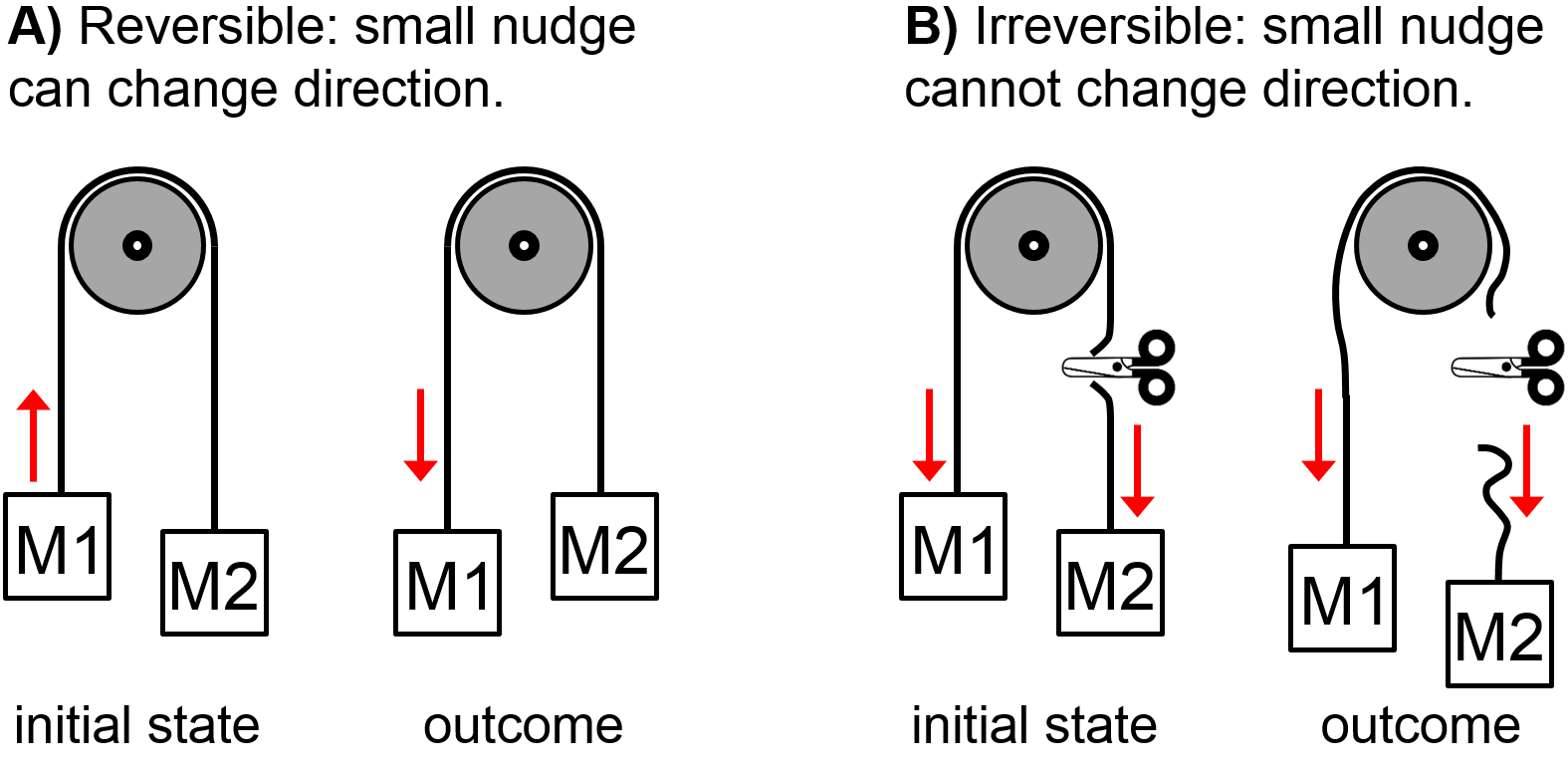
Fig. 2.7 Pulley analogy for reversibility with two equal masses M1 and M2. In A), mass M1 is initially moving slowly downward but a small nudge in the opposite direction can change the direction of motion. This is an example of a reversible process. In B), scissors have cut the rope and both masses are initially moving downward. A small nudge in the opposite direction will not change the direction of motion. This is an example of an irreversible process. (Figure adapted from [17].)

2.8.1. Principle of Maximum Work

A reversible process is one that occurs very slowly and at equilibrium at all points during the process. We can apply this processes to gas expansions or compressions to see what are some of the consequences of being reversibile or not.

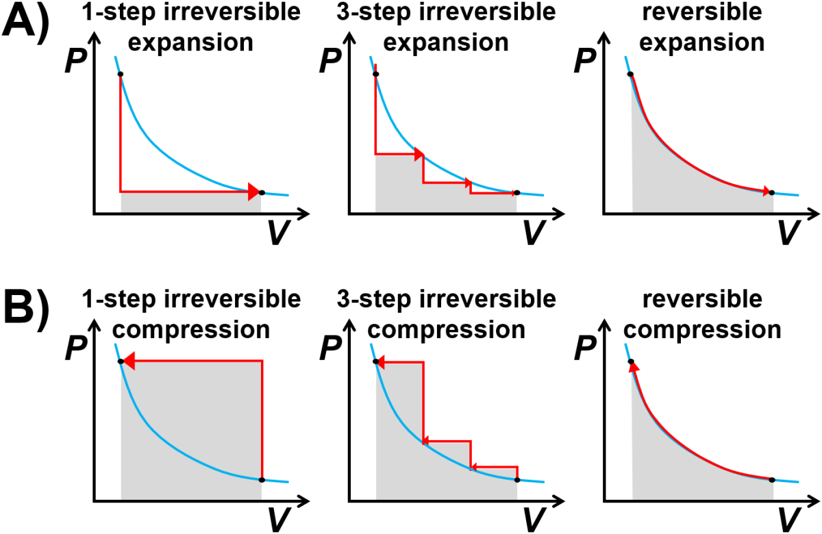
Fig. 2.8 Principle of maximum work applied to A) expansion and B) compression of an ideal gas. The blue curve represents an ideal gas ‘isotherm’ curve with \(P=nRT/V\).

Sudden vs Gradual Expansion. Imagine expanding an ideal gas between the same initial and final states but using different paths (Fig. 2.8 A). In the first path the external pressure is dropped down instantly to the final pressure in what is known as a single irreversible step. The work done on the gas is negative, which is shown in the graph as the gray area. In the second path, the gas is expanded in a series of three sudden, irreversible steps where the pressure is ramped down three times to the final pressure. The magnitude of the work done is larger since the portion of the expansion occurring at a higher pressure leads to a larger area. In the third path, the gas is expanded gradually and reversibly (such that \(P_\textrm{system} \approx P_\textrm{surroundings}\) at all times) and this yields the maximum usable work from the system.

Sudden vs Gradual Compression. How do irreversible and reversible processes look for compression? For a single-step irreversible compression, a sudden increase in the external pressure requires a large amount of external work to compress the system. A three-step irreversible compression, with three, smaller sudden pressure increases, requires less external work, while a slow, reversible compression requires the minimum amount of work necessary.

While a truly reversible process would be hard or perhaps impossible to achieve, some well-designed, sufficiently processes can come close. It may be more useful to consider a reversible process as the limit of a slow, gradual process that occurs at equilibrium. We can see that when that limit is achieved for a gas, the magnitude of the work is equal for expansion or compression, but irreversible processes the magnitude of work for compression is larger than the magnitude of work for expansion.

I have noticed that students sometimes find the the abrupt vertical jumps in the \(PV\) diagrams in Fig. 2.8 to be confusing and I have a few comments. First of all, note that a veritical jump at constant volume requires there to be a temeperature change, such as a sudden heating process. Second, for real processes, the jumps may be a little bit more rounded and that deviate from the blue isotherm curves but don’t necessarily follow perfectly vertical or horizontal paths on the \(PV\) diagram. Better yet, think of these as representative examples of an irreversible process with the result that as the process becomes more gradual, the magnitude of work for expansion approaches that of the magnitude of work for compression.

2.9. Revisiting Energy for Gradual Changes

In thermodynamics we sometimes are interested in discrete changes that we indicate as discrete by using the symbol \(\Delta\). In other cases, we may want to study infitesimal changes that we can integrate over a path of interest in order to calculate something and we tend to use notation such as you are used to for derivatives (\(dF/dx\)), partial derivatives (\(\partial F/\partial x\)), or differentials (such as \(dF=2dx+xdy\)) that tell us how small changes in one variable relate to small changes in another variable. Here we will revisit the quantities we have learned, above, for energy in the first law, now in the form of differentials (see Table 2.5).

Table 2.5 Summary of symbols or equations for discrete changes (final minus initial) or infitesimal changes.

Symbol/Equation	Discrete Change	Infinitesimal Change
Change	\(\Delta\)	\(d\) or \(\partial\)
\(PV\) work	\(w=-\int P_\textrm{ext}dV\)	\(dw=-P_\textrm{ext}dV\)
Heat Capacity (const. \(P\))	\(q=n\overline{C}_P\Delta T\)	\(dq=n\overline{C}_PdT\)
Heat Capacity (const. \(V\))	\(q=n\overline{C}_V\Delta T\)	\(dq=n\overline{C}_VdT\)
First Law	\(\Delta U = q + w\)	\(dU = dq + dw\)
Ideal Gas \(\Delta U\)	\(\Delta U = n C_V \Delta T\)	\(dU = n C_V dT\)
Ideal Gas \(\Delta H\)	\(\Delta H = n C_P \Delta T\)	\(dH = n C_P dT\)

2.10. Key Gas Processes and the First Law

Ideal gas calculations are valuable in learning thermodynamics because they are relatively simple and can be performed exactly in many cases. Although their are a large number of variations that are possible, I will review in this section a subset of classic problems that illustrate many key ideas. We will return to gas calculations in subsequent sections including after entropy and Gibbs free energy are introduced.

I have two pieces of general advice for performing these sorts of calculations. First, is that you should read the problem carefully so that you understand what is happening, what you know, and what you are supposed to calculate. Here the subsection title indicates the sort of process but note that for homework, quiz, or exam problems you would just be given the problem text and would need to figure out if the process is irreversible or isothermal, etc., by carefully reading the problem statement. Slowly or gradually will mean reversible, whereas suddenly or instantly will mean irreversible. Sometimes you will have to read the problem wording carefully to figure out if a process is reversible or irreversible, such as whether expansion is against a constant pressure (irreversible) or a pressure that changes together with the system pressure. Many key situations encountered in these problems are summarized in Table 2.6.

In order to help process the information provided in the problem statement, I usually like to draw a diagram where I indicate this information, and I think this can help many students. Second, a wonderful exercise before doing the exact calculations for many of these problems is to see wehther you can determine the signs of the various quantities requested without performing full calculations. It helps you quickly test your conceptual understanding and can also help you check for mistakes.

I have a final note. Unless indicated otherwise, an ideal gas will be assumed to mean a monatomic gas that obeys the gas law, \(PV=nRT\), has \(\overline{C}_V=\frac{3}{2}R\), \(\overline{C}_P=\frac{5}{2}R\), \(\Delta U=nC_V R\), and \(\Delta H=nC_P R\) regardless of the path. Some sources refer to a ‘diatomic ideal gas’ which still follows the ideal gas law but which has \(\overline{C}_V=\frac{5}{2}R\) and \(\overline{C}_P=\frac{7}{2}R\) (while still being the case that \(\Delta U=nC_V R\) and \(\Delta H=nC_P R\)).

Table 2.6 Summary of various processes or conditions and their consequences.

Process/Condition	Consequence
Constant volume	\(dV=0\) so that \(w=0\)
Constant temperature	\(dT=0\) so that \(\Delta U = \Delta H = 0\)
Constant pressure	\(dP_\textrm{sys}=0\) so that \(\Delta H=q\)
Adiabatic	\(dq=0\) so that \(dU=dw\) and \(q=0\) so that \(\Delta U = w\)
Free expansion	\(P_\textrm{ext}=0\) so that \(w=0\), \(\Delta T=0\)
Reversible volume change	\(P_\textrm{ext}=P_\textrm{sys}\) (but may not be constant)
Irreversible volume change	Often this means \(P_\textrm{ext}=P_\textrm{final}=\textrm{constant}\)
Slowly or gradually	Typically means the process is reversible

2.10.1. Irreversible Adiabatic Process

1 mol of ideal gas initially at 1 atm and 400 K expands adiabatically against a constant and final pressure of 0.5 atm. Calculate \(q\), \(w\), \(\Delta U\), and \(\Delta H\).

First, let’s draw a picture to indicate what we know from reading the problem statement.

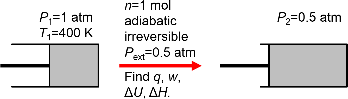
Second, let’s think about how we will calculate the items requested in the problem. Well, the process is indicated as adiabatic so we already know without doing any calculation that \(q=0\) and we know that the first law will become \(\Delta U = w\). We also know that for this (assumed monatomic) ideal gas \(\Delta U = \frac{5}{3} \Delta H\). In short, if we can calculate \(\Delta U\) we can easily calculate \(w\), \(\Delta U\), and \(\Delta H\). We are not given enough information about the initial and final states to calculate \(\Delta T\) directly (if both \(T_1\) and \(T_2\) were provided) or indirectly (if we had enough information to use the ideal gas law to calcualte \(T_1\) and \(T_2\) from knowledge of \(P\), \(V\), \(n\) for initial and final states) so things will get a little more involved. Our strategy will be to try to calculate both \(\Delta U\) and \(w\) in terms of the unknown final temperature and then use the resulting equation to solve for the final temperature.

Before we do the exact calculation, let’s try to predict signs. We can expect that work on the surroundings would be negative since expansion means \(\Delta V>0\) and \(w=-\int P_\textrm{ext}dV\). The process is adiabatic with \(q=0\), so the first law turns into \(\Delta U=w\), and since \(w<0\), we expect that \(\Delta U<0\). Similarly, since for an (monatomic) ideal gas it is always true that \(\Delta H = \frac{5}{3}\Delta U\) then we expect \(\Delta H<0\) as well.

Now, here here goes with the detailed calculation.

First, here is \(\Delta U\).

\[\Delta U = \int_{T_1}^{T_2}n\overline{C}_VdT=n\overline{C}_V(T_2-T_1)=\frac{3}{2}nR(T_2-T_1)\]

Next, here is \(w\).

\[\begin{split}w &= -\int_{V_1}^{V_2}P_\textrm{ext}dV = -\int_{V_1}^{V_2}P_2dV = -P_2(V_2-V_1) \\ &=-P_2\left( nR\frac{T_2}{P_2} - nR\frac{T_1}{P_1} \right) =-nRP_2\left( \frac{T_2}{P_2} - \frac{T_1}{P_1} \right) = -nR\left( T_2 - \frac{T_1}{2} \right)\end{split}\]

Next we will equate our reuslts for \(\Delta U\) and \(w\) and simplify.

\[\begin{split}\frac{3}{2}nR(T_2-T_1) &= -nR\left( T_2 - \frac{T_1}{2} \right) \\\end{split}\]

Multiplying both sides by \(nR/2\) yields

\[3T_2 - 3T_1 = -2T_2 + T_1\]

which can be solved to give

\[T_2 = \frac{4}{5}T_1 = 320 \textrm{ K}\]

After this, we can easily calculate the remaining quantities \(w\), \(\Delta U\), and \(\Delta H\).

\[\begin{split}\Delta U &= n\overline{C}_V\Delta T = n\frac{3}{2}R(T_2 - T_1)= 1.5 \textrm{ mol }8.31\frac{\textrm{J}}{\textrm{K mol}}(-80 \textrm{ K})=-998 \textrm{ J} \\ \Delta H &= \frac{5}{3}\Delta U = -1663 \textrm{ J} \\ w &= \Delta U = -998 \textrm{ J} \\\end{split}\]

The signs we predicted all agree with our detailed calculation, as expected.

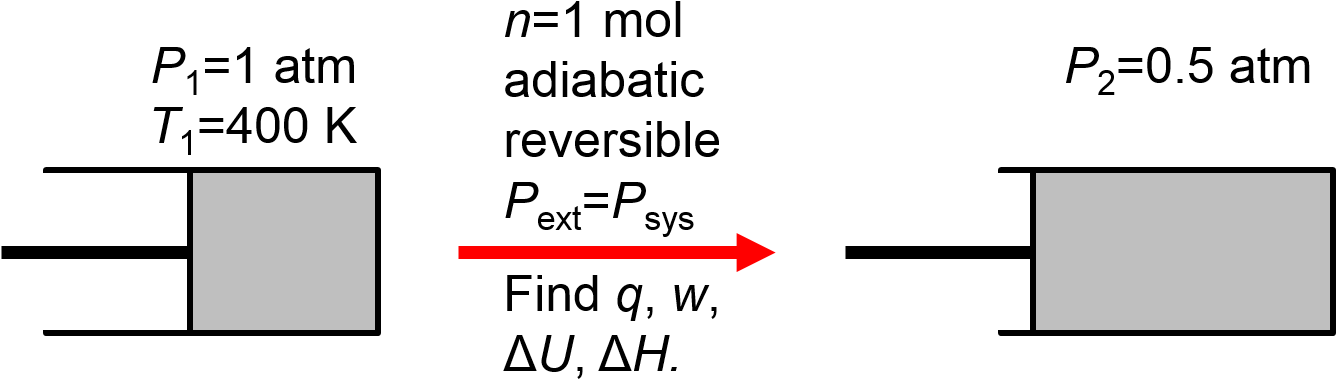
2.10.2. Reversible Adiabatic Process

1 mol of ideal gas initially at 1 atm and 400 K expands adiabatically and reversibly against an external pressure that starts at 1 atm and slowly decreases to 0.5 atm. Calculate \(q\), \(w\), \(\Delta U\), and \(\Delta H\).

Ok, this is a reversible process, meaning here that the system pressure and surroundings pressure are always equal to each other. Also note that the surroundings/system pressure is changing, even though it is not stated why or how this happens. How could you do this in real life? What if you inserted some gas in a frictionless piston that is thermally insulated and then walked with the piston up a tall hill from sea level to 25,000 feet? In that case, the surroundings pressure would slowly decrease and would always match the system pressure. It might seem somewhat artificial, although if the mass of gas were a cloud that blows against a mountain range and rises upwards to an altitude of lower pressure, then perhaps it doesn’t seem so far-fetched anymore.

First, let’s draw a picture to indicate what we know from reading the problem statement.

Before we do the exact calculation, let’s try to predict signs. Well, the path is still an adiabatic expansion. We expect the same signs here as for the irreversible expansion example in Section 2.10.1 since the reasoning in that problem did not depend on whether the process was reversible or irreversible. So, again we predict \(\Delta V>0\) and \(w=-\int P_\textrm{ext}dV\), \(q=0\), \(\Delta U<0\), and \(\Delta H<0\).

As with the irreversible expansion example in Section 2.10.1, because the process is adiabatic, we know that \(q=0\) and \(\Delta U = w\). Similarly to the irreversible case, once we calculate \(\Delta U\) we can easily calculate \(w\) and \(\Delta H\) but we don’t directly or indirectly konw \(T_1\) and \(T_2\) yet so we will again try to calculate both \(\Delta U\) and \(w\) in terms of the unknown final temperature and then use the resulting equation to solve for the final temperature. However we must be careful here. Let’s take a closer look to see why.

We could try to proceeded as before using \(\Delta U = w\) and then separately calculating \(\Delta U\) and \(w\) but we will encounter a problem trying to calculate \(w\) in this case.

\[w = -\int_{V_1}^{V_2}P_\textrm{ext}dV = -\int_{V_1}^{V_2}P_\textrm{sys}dV = -\int_{V_1}^{V_2}\frac{nRT}{V}dV\]

but we can’t calculate the above integral since both `T` and `V` are changing! We will need to take a different approach, and this gives us an opportunity to use the differentials for energy discussed in Section 2.9.

This time, we will use the differential form of the first law which states that \(dU=dq+dw\) and for and adiabatic system becomes \(dU=dw\). The differential for work is \(dw=-P_\textrm{ext}dV\) and for ideal gases the internal energy differential is \(dU=n\overline{C}_VdT\). We can put these equations together to get the following.

\[n\overline{C}_VdT = dU = dw = -P_\textrm{ext}dV=-P_\textrm{sys}dV\]

We can use the left-most and right-most sides of the above equation along with \(P_\textrm{sys}=nRT/V\) to get

\[n\overline{C}_VdT = -\frac{nRT}{V}dV\]

Next, we will prepare to integrate both sides, but first take a close look. Temperature appears both on the left an dthe right sides of the differential. We need to first separate variables to collect all the terms containing a \(T\) on the left side of the equation which will be integrated with respect to \(T\) and all the \(V\) terms on the right. We can do this, after canceling out the \(n\) terms on both sides and dividing both sides by \(R\) to get

\[\frac{\overline{C}_V}{R}\frac{dT}{T} = -\frac{dV}{V}\]

For a (monatomic) ideal gas, \(\overline{C}_V=\frac{3}{2}R\) so the above differential becomes

\[\frac{3}{2}\frac{dT}{T} = -\frac{dV}{V}\]

We can straightforwardly integrate both sides now that the variables are properly separated, taking care to use corresponding limits of integration.

\[\frac{3}{2}\int_{T_1}^{T_2}\frac{dT}{T} = -\int_{V_1}^{V_2}\frac{dV}{V}\]

This gives us

\[\frac{3}{2}\ln\frac{T_2}{T_1} = -\ln\frac{V_2}{V_1}\]

This is good progress but we are trying to solve for the final temperature rather than volumes so we can use \(PV=nRT\) to work with the volume terms. In the line, below, I also use the fact that for this problem, \(\frac{P_2}{P_1}=\frac{1}{2}\).

\[-\ln\frac{V_2}{V_1} = \ln\frac{V_1}{V_2} = \ln\frac{nRT_1P_2}{P_1nRT_2} = \ln\frac{T_1P_2}{P_1T_2} = \ln\frac{T_1}{2T_2}\]

Putting the above two expressions together gives us

\[\frac{3}{2}\ln\frac{T_2}{T_1} = \ln\frac{T_1}{2T_2}\]

which is a single equation with a single unknown, \(T_2\), so in principle we can calculate \(T_2\), however, it takes a little more work. We will use some logarithm algebra properties for this.

\[\frac{3}{2}\ln\frac{T_2}{T_1} = \ln\left(\frac{T_2}{T_1}\right)^{3/2} = \ln\frac{T_1}{2T_2}\]

Next, we can exponentiate the middle and right terms in the above equation to get rid of the natural logarithm

\[\left(\frac{T_2}{T_1}\right)^{3/2} = \frac{T_1}{2T_2}\]

and we can solve for \(T_2\) to get

\[T_2 = \frac{T_1}{2^{2/5}} = 0.758 T_1 = 303 \textrm{ K}\]

With knowledge of the initial and final temperatures we can now calculate \(\Delta U\) (and \(w\)) as

\[\Delta U = w = n\overline{C}_V\Delta T = n\frac{3}{2}R(0.748T_1 - T_1) = -1207 \textrm{ J}\]

and \(\Delta H\) as

\[\Delta H = \frac{5}{3}\Delta U = -2011 \textrm{ J}\]

2.10.3. Free Expansion

2 moles of ideal gas initially at 275,00 Pa and 360 K is expanded against a vacuum to a final volume of 0.5 \(\textrm{m}^3\). Calculate \(q\), \(w\), \(\Delta U\), \(\Delta H\), and \(\Delta T\).

Once again, let’s draw a picture to indicate what we know from reading the problem statement.

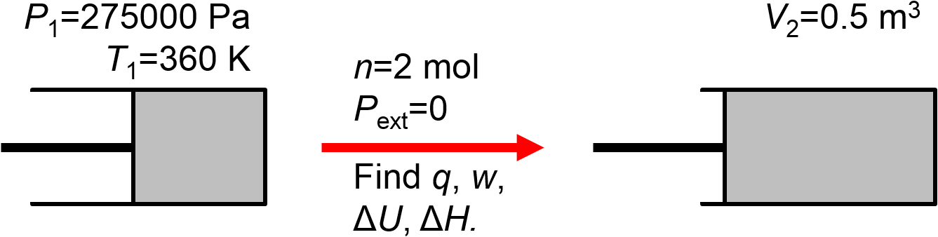
For this problem, it turns out that we can determine all of the desired quantities relatively easily from simple consideration of the provided information. First of all, the external pressure is zero. Since it is not possible to do work against a vacuum, based on \(w=-\int P_\textrm{ext}dV\), we will have \(w=0\). The gas is surrounded by a vacuum and there is nothing in the surroundings that can exchange heat with the system, so we know that \(q=0\). The first law tells us that \(\Delta U = q + w\) so it must also be the case that \(\Delta U = 0\) and therefore that \(\Delta T=0\) and \(\Delta H = 0\). None of the requested quantities change. So what does change? Well, as the volume increases, if temperature is held constant, then it must be the case that the pressure decreases.

Let’s also take a moment to think about this process from a physical perspective. The kinetic theory of gases showed us that the temperature of a gas is related to the average translational kinetic energy and that this is a function of the average speed of the gas particles. With that in mind, imagine gas particles that are initially zipping around and bouncing off the container walls just as the gas is allowed to expand into a vacuum, as if one wall of the container suddenly disappeared. There is nothing to slow down the gas particles, and they will keep traveling the same speed. If they have the same speed then they will have the same the same kinetic energy and the same temperature. In that case, the temperature doesn’t change. From there, we can easily conclude that the internal energy and enthalpy of the gas also don’t change.

2.11. Additional Problems

2.11.1. Practice Calculating Signs of Work, Energy, Enthalpy

Gas process

Question: An ideal gas is compressed adiabatically and reversibly. Select whether the indicated thermodynamic quantities are zero, greater than zero, or less than zero: \(q\), \(w\), \(\Delta U\), \(\Delta H\), \(\Delta P\), and \(\Delta T\).

Answer:

The process is adiabatic, which by definition means that \(q=0\). Since the gas is compressed, \(\Delta V<0\) and since \(w=-\int PdV\), we can conclude \(w>0\). By the first law, \(\Delta U = q + w\), and since \(q=0\) and \(w>0\), we can conclude \(\Delta U > 0\). Since for an ideal gas, it is always true that \(\Delta H = \frac{5}{3}\Delta U\), we can conclude that \(\Delta H > 0\). Since \(\Delta U > 0\) and since it is always true for an ideal gas that \(\Delta U = n\frac{3}{2}R\Delta T\), it must be the case that \(\Delta T>0\). It turns out that \(\Delta P > 0\); by solving the adiabatic expansion (try it!), it can be shown that \(P_2 = P_1\left(\frac{T_2}{T_1}\right)^{\frac{5}{2}}\), and since \(T_2>T_1\), we can see that the pressure increases (or that \(P_2>P_1\)).

Methane Combustion

Question: \(\ce{CH4}\) reacts exothermically (\(q<0\)) with \(\ce{O2}\) to form only \(\ce{CO2}\) and \(\ce{H2O}\) at an initial pressure of 1.2 atm and an initial temperature of 315 K. After the reaction is complete, the products return to 1.2 atm and 315 K. All reactants and products are gases and you may use \(PV=nRT\) to calculate volume changes. Determine whether \(w\), \(\Delta U\), and \(\Delta H\) are each \(>0\), \(<0\), \(=0\).

Answer:

The balanced reaction for the complete combustion of methane by oxygen is shown below.

\(\ce{CH4 + 2O2 -> CO2 + 2H2O}\)

The change in the number of moles is zero so there is no volume change, \(\Delta V=0\) and therefore \(w=0\). Since \(q<0\) and \(\Delta U = q + w = q\), it must be the case that \(\Delta U<0\). Also, since \(\Delta H = \Delta U + \Delta (PV)\), with \(\Delta (PV)=0\), it must be that \(\Delta H <0\).

Methanol Combustion

Question: \(\ce{CH3OH}\) reacts exothermically (\(q<0\)) with \(\ce{O2}\) to form only \(\ce{CO2}\) and \(\ce{H2O}\) at an initial pressure of 0.9 atm and an initial temperature of 300 K. After the reaction is complete, the products return to 0.9 atm and 300 K. All reactants and products are gases and you may use \(PV=nRT\) to calculate volume changes. Determine whether \(w\), \(\Delta U\), and \(\Delta H\) are each \(>0\), \(<0\), or \(=0\).

Answer:

The balanced reaction for the complete combustion of methanol by oxygen is shown below.

\(\ce{CH3OH + \frac{3}{2}O2 -> CO2 + 2H2O}\)

The change in the number of moles is \(+0.5 \textrm{mol}\) so the volume increases, \(\Delta V>0\) and therefore \(w<0\). Since \(q<0\) and \(\Delta U = q + w\), it must be the case that \(\Delta U<0\). Also, since \(\Delta H = \Delta U + \Delta (PV)\), with \(\Delta (PV)<0\), it must be that \(\Delta H <0\).

2.11.2. Heat Capacity

True/False

Question: 1 kg of solid water at -18.7 °C is added to 1 kg of liquid water at 30.2 °C. After the system reaches thermal equilibrium, how many moles of liquid water are present? The heat capacity of liquid water is \(C_{\textrm{Liq}} = 75.3 \frac{\textrm{J}}{\textrm{K mol}}\), the heat capacity of solid water is \(C_{\textrm{Sol}} = 38.1 \frac{\textrm{J}}{\textrm{K mol}}\), and the enthalpy of fusion of water is \(\Delta H_\textrm{fus}=6010 \frac{\textrm{J}}{\textrm{mol}}\).

Answer:

Let’s first compare some quantities to determine what phase(s) remain. Note that for water, 1 kg = 55.6 mol.

Cooling liquid water from 30.2 °C to 0 °C would release heat.

\[q_{\textrm{Liq}}=55.6 \textrm{ mol} \times 75.3 \frac{\textrm{J}}{\textrm{K mol}} \times \left(-30.2 \textrm{ K} \right) = -126.3 \textrm{ kJ}\]

Heating ice from -18.7 °C to 0 °C would absorb some of the heat relased when the liquid water is cooled. So we know that all of the ice will heat to at least 0 °C.

\[q_{\textrm{Sol}}=55.6 \textrm{ mol} \times 38.1 \frac{\textrm{J}}{\textrm{K mol}} \times \left(+18.7 \textrm{ K} \right) = 39.6 \textrm{ kJ}\]

Melting 1 kg ice would require quite a bit of heat, more than can be provided by the cooling of the liquid water.

\[q_{\textrm{melt all ice}}=55.6 \textrm{ mol} \times 6.01 \frac{\textrm{kJ}}{\textrm{mol}} = 334.1 \textrm{ kJ}\]

Therefore only some of the ice will melt and the final composition is a mixture of solid and liquid water at 0 °C. How much of each is present? Well, the melting of the ice and cooling of the water left \(86.7 \textrm{ kJ}\) of heat to melt ice, or

\[n_{\textrm{melt}}=\frac{86.7 \textrm{ kJ}}{6.01 \textrm{ kJ/mol}}=14.4 \textrm{ mol}\]

so that there are \(55.6 \textrm{ mol} + 14.4 \textrm{ mol} = 70.0 \textrm{ mol}\) liquid water present and \(55.6 \textrm{ mol} - 14.4 \textrm{ mol} = 41.6 \textrm{ mol}\) solid water present.

2.11.3. General Questions

True/False

Question: Choose True or False for each of the statements below.

1. The enthalpy change of a system is greater than its internal energy for all processes.

2. An expanding gas always has work that is <0 J.

3. An ideal gas that expands against constant pressure has a change in internal energy that is given by \(\Delta U = nC_V\Delta T\), where \(C_V=\frac{3}{2}R\) is the constant volume heat capacity.

Answer:

1. False. Any isothermal process with an ideal gas will have \(\Delta H = \Delta U = 0\).

2. False. Expansion of an ideal gas into vacuum has \(w=0\) since \(P_{ext}=0\).

3. True. \(\Delta U = n\frac{3}{2}R\Delta T=nC_V\Delta T\) is always true for an ideal gas.

Bond Dissociation Enthalpy

Question: Use the information in Table 2.4 to answer the questions, below.

1. What is the bond dissociation enthalpy for a C-F bond?

2. What is the bond dissociation enthalpy for a B-F bond?

3. Which bond is stronger, C-F or B-F?

Answer:

The general equation we will use is shown below.

\[\sum \textrm{BDE}_\textrm{all bonds} = \sum \Delta H^\circ_\textrm{form., atoms} - \Delta H^\circ_\textrm{form., molecule}\]

1. There are four C-F bonds in \(\ce{CF4}\) and we can use that to calculate \(\textrm{BDE}_{\textrm{C-F}}\).

\[\begin{split}\textrm{BDE}_\textrm{C-F} &= \frac{1}{4}\left( \Delta_f H^\circ_\textrm{C,atom} + 4\Delta_f H^\circ_\textrm{F,atom} - \Delta_f H^\circ_{\ce{CF4}\textrm{,mol.}} \right) \\ &= \frac{1}{4}\left( 716.7 \textrm{ kJ/mol} + 4\times79 \textrm{ kJ/mol} + 925 \textrm{ kJ/mol} \right) \\ &= 489 \textrm{ kJ/mol}\end{split}\]

2. There are three B-F bonds in \(\ce{BF3}\) and we can use that to calculate \(BDE_{\textrm{B-F}}\).

\[\begin{split}\textrm{BDE}_\textrm{B-F} &= \frac{1}{3}\left( \Delta_f H^\circ_\textrm{B,atom} + 3\Delta_f H^\circ_\textrm{F,atom} - \Delta_f H^\circ_{\ce{BF3}\textrm{,mol.}} \right) \\ &= \frac{1}{3}\left( 562.7 \textrm{ kJ/mol} + 3\times79 \textrm{ kJ/mol} + 1037 \textrm{ kJ/mol} \right) \\ &= 612 \textrm{ kJ/mol}\end{split}\]

3. The above calcalations show that a B-F bond (612 kJ/mol) is stronger than a C-F bond (489 kJ/mol).