4. Free Energy and Equilibrium
The second law tells us whether a process/reaction is spontaneous or not, but it is inconvenient to have to calculate \(\Delta S\) for both the system and the surroundings in order to determine whether or not \(\Delta S_\textrm{univ}>0\). Here we will introduce a new measure of thermodynamic energy that already factors in the entropy changes of the surroundings—the Gibbs free energy \(G\), which is a sort of combination of the first and second laws. It is particularly nice since many reactions of interest occur at constant pressure and temperature, and we can just look at the change in Gibbs free energy, \(\Delta G\) to see if the process is spontaneous. While we are at it, I will also introduce the Helmholtz free energy \(A\) which is similar but is designed for constant volume and temperature. Importantly, both \(G\) and \(A\) are state functions and they are tabulated as energies of formation relative to standard state, just like \(H\) and \(S\).
4.1. Gibbs Free Energy
The Gibbs free energy is named after the great American scientist Josiah Willard Gibbs (who also coinvented vector calculus and statistical mechanics, among other achievements). Let’s see how it works.
The second law tells us that a process is spontaneous if \(\Delta S_\textrm{univ}>0\) which we can assess by calculating
For processes that occur at constant temperature, the suroundings may be treated reversibly, so that
where the second step used the fact that heat gained by the system is equal to heat lost by the surroundings, or \(q_\textrm{sys}=-q_\textrm{surr}\). Next, if the process also occurs at constant pressure, where \(\Delta H_\textrm{sys} = q_\textrm{sys}\), then the above equation becomes
If we substitute Eq. (4.2) into Eq. (4.1) and multiply both sides by \(-T\) we obtain
Notice in the above equation that we have been able to calculate \(\Delta S_\textrm{univ}\) from consideration of properties of the system, namely, \(\Delta S_\textrm{sys}\) and \(\Delta H_\textrm{univ}\). This means that for processes that occur at constant temperature and pressure, it is sufficient to calculate \(\Delta S_\textrm{univ}\) using only properties of the system in order to determine whether a process is spontaneous or not.
Now when we look at the definition of the Gibbs Free Energy, a state function, using
we can see that at constant temperature we have
Putting this all together, we can see that the mathematical definition Eq. (4.3) leads to the quantity \(\Delta G\) that, for constant temperature and pressure processes, predicts whether a process will be spontaneous, reversible, or impossible. As shown in Table 4.1 spontaneous processes have \(\Delta G<0\) while \(\Delta S_\textrm{univ}>0\).
Finally, what about the term energy? Well, a convenient interpretation of the Gibbs free energy is that it is the maximum amount of non-pressure-volume work that may be performed by a system at constant temperature and pressure.
4.2. Helmholtz Free Energy
We saw in Section 4.1 that the Gibbs free energy provided a convenient way to predict whether a process will be spontaneous or not provided that the process occurs at constant temperature and pressure. What if a process occurs under different experimental conditions? If a process occurs at constant temperature and volume, we can use a different measure of free energy, called the Helmholtz free energy, that under these conditions is equal to \(\Delta S_\textrm{univ}\).
The Helmholtz free energy, \(A\), is also a state function, and is named after the Germany physicist (plus all-around genious) Hermann von Helmholtz. It is defined as
Once again, for a constant temperature process, the surroundings can be treated reversibly to give
Now for a constant volume process, no pressure-volume work may be done, so that the first law becomes \(\Delta U_\textrm{sys}=q_\textrm{sys}\), and we obtain
Multiplying the above by \(-T\), we obtain
Returning to the definition of the Helmholtz free energy, for a constant temperature process we can see that
Thus, for processes that occur at constant temperature and volume, it is clear that the change in Helmholtz free energy is equivalent to \(-T\Delta S_\textrm{univ}\) and is therefore able to predict whether a process is spontaneous or not. Analogous with the Gibbs free energy, the Helmholtz free energy is the maximum amount of work that may be done by the system under conditions of constant temperature and volume. It turns out that these conditions are probably less common to most chemists and biochemists than constant temperature and pressure, so we won’t heavily use the Helmholtz free energy, but it is nonetheless a good tool to have in our toolkit. Table 4.1 provides a brief summary of the conditions for spontaneity for \(\Delta S_\textrm{univ}\), \(\Delta G\), and \(\Delta A\).
Process |
Always |
Constant \(T\) and \(P\) |
Constant \(T\) and \(V\) |
|---|---|---|---|
spontaneous |
\(\Delta S_\textrm{univ}>0\) |
\(\Delta G<0\) |
\(\Delta A<0\) |
reversible |
\(\Delta S_\textrm{univ}=0\) |
\(\Delta G=0\) |
\(\Delta A=0\) |
impossible |
\(\Delta S_\textrm{univ}<0\) |
\(\Delta G>0\) |
\(\Delta A>0\) |
4.3. Free Energy Example Problems
Let’s get some practice using the Gibbs free energy for some processes (at constant \(P\) and \(T\))) to predict whether reactions are spontaneous. While doing calculating \(\Delta G=\Delta H - T\Delta S\), we will pay some attention to the signs of the terms \(\Delta H\) or \(T\Delta S\) in order to determine whether the process is enthalpically driven (\(\Delta H<0\)), enthalpically opposed (\(\Delta H>0\)), entropically driven (\(-T\Delta S<0\)), or entropically opposed (\(-T\Delta S>0\)), and so forth. Of course, in these discussions, please keep in mind that all spontaneous reactions are in fact driven by increases in the entropy of the universe, but it can be insightful to determine whether that entropy increase may come from enthalpy changes of the system or entropy changes of the system.
Example 1. Calculate \(\Delta G\) for the freezing of supercooled water at 263 K, 1 atm. Is the process spontaneous? Is it driven or opposed for both enthalpy change and entropy change?
We already determined the enthalpy of fusion of supercooled water at 263 K to be \(\Delta H_\textrm{fus,263K}=5640 \frac{\textrm{J}}{\textrm{mol}}\) (Section 2.5) and we also already determined the entropy of fusion of supercooled water at 263 K to be \(\Delta S_\textrm{fus,263K}=-20.6 \frac{\textrm{J}}{\textrm{K mol}}\) (example problem). These were both calculated using alternate path strategies. Now we can simply look at the value of \(\Delta G\). Note that, as always, we will manually enter the sign of the enthalpy term, which is negative since upon freezing the system loses heat to the surroundings.
The negative value of \(\Delta G\) tells us that the process is spontaneous. We can look at the two separate temrs to see that the system is enthalpically driven but entropically opposed. That is, the release of heat to the surroundings upon freezing increases the entropy of the surroundings, but the negative value of \(\Delta S\) upon freezing tends increase the value of \(\Delta G\) but not to a sufficient level that it caused \(\Delta G\) to become positive overall.
Practice \(\Delta G\) calculation for a phase change.
Question: What is the value of \(\Delta G\) for the boiling of superheated water at 383 K, 1 atm? Is the process spontaneous? Is it driven or opposed for both enthalpy change and entropy change? You may use the values \(\Delta H_\textrm{vap,383K}=40320 \frac{\textrm{J}}{\textrm{mol}}\) and \(\Delta S_\textrm{vap,383K}=107.6 \frac{\textrm{J}}{\textrm{K mol}}\).
Answer:
The process is overall spontaneous, with \(\Delta G = -890.8 \frac{\textrm{J}}{\textrm{mol}}\), but this time it is the entropy change of vaporiztaion that drives the process and it is opposed by the positive enthalpy change but not to an extent that it caused \(\Delta G\) to become positive overall.
Example 2. Calculate \(\Delta G\) for the freezing of water at 273 K, 1 atm. Is the process spontaneous? Is it driven or opposed for both enthalpy change and entropy change? For the freezing of water at 273 K, 1 atm, use the values \(\Delta H_\textrm{fus,273K}=6010 \frac{\textrm{J}}{\textrm{mol}}\) and \(\Delta S_\textrm{fus,273K}=22 \frac{\textrm{J}}{\textrm{K mol}}\).
You may have obtained a value of \(-4 \frac{\textrm{J}}{\textrm{mol}}\) in your calculator and may be wondering why I have approximated it as zero. Well, the small remaining value is essentially a small numerical error due to the imprecision of our input values. We know that water freezes at equilibrium at 273 K, 1 atm, and therefore the process must have a value of \(\Delta G=0\). We are actually subtracting two relatively large-ish numbers and would actually obtain a value of \(\Delta G = 0\) if we used more precise values for \(\Delta H_\textrm{fus,273K}\) and \(\Delta S_\textrm{fus,273K}\). The value of zero obtained for \(\Delta G\) occurs when the enthalpy and entropy terms cancel each other out (that is, the process is enthalpically driven and entropically opposed).
Example 3 Calculate the enthalpy change for the reaction shown below at 298 K. Is the process spontaneous? Is it driven or opposed for both enthalpy change and entropy change?
Substance |
\(\Delta_f H^\circ \frac{\textrm{kJ}}{\textrm{mol}}\) |
\(S ^\circ \frac{\textrm{J}}{\textrm{K mol}}\) |
|---|---|---|
\(\ce{Ba(OH2)*8H2O(s)}\) |
-3,342 |
427 |
\(\ce{NH4Cl(s)}\) |
-314 |
95 |
\(\ce{BaCl2*2H2O(s)}\) |
-1,460 |
203 |
\(\ce{NH3(aq)}\) |
-80 |
111 |
\(\ce{H2O(l)}\) |
-285 |
70 |
We can calculate the enthalpy change for the reaction using Eq. (2.2) and the entropy change for the reaction using Eq. (3.4) using the information in Table 4.2. Doing so, we obtain
From these values, we can calculate the value of \(\Delta G\).
Since \(\Delta G_\textrm{rxn}<0\), this reaction is spontaneous. In this instance, the enthalpy term is positive so it is enthalpically opposed, but the entropy term \(- T\Delta S_\textrm{rxn}\) is negative and (entropically driven) and sufficiently large to make \(\Delta G_\textrm{rxn}\) negative overall. This is an example of a spontaneous endothermic reaction. Note that in many settings, endothermic (or exothermic) reactions may not maintain a constant temperature. They may at first cool (or heat) themselves up before their temperature re-equilibrates with the surroundings. A spontaneous endothermic reaction like this one, if performed in the lab by mixing chemicals in an open beaker would likely feel very cold to the touch during the reaction.
4.4. Free Energy Under Nonstandard Conditions
If you are considering a chemical reaction at constant temperature and pressure and you are provided with or can easily look up \(\Delta H\) and \(\Delta S\) at that temperature and pressure then you can simply use these in \(\Delta G=\Delta H - T\Delta S\). However, in many cases, reactions will be considered under conditions that are at different temperature or pressure. The reaction of interest may still occur at a constant temperature or pressure, but if these are different than the conditions at which \(\Delta H\) and \(\Delta S\) are available, then it is useful to have some tools available for calculating \(\Delta G\) at these alternative conditions. In this section, we will look at two approaches to determining \(\Delta G\) under conditions different from the tabulated values of \(\Delta H\) and \(\Delta S\).
4.4.1. Estimate Free Energy for New Temperature
A simple approximation that is suitable in some situations is to estimate \(\Delta H\) and \(\Delta S\) as constant over a temperature range and to calculate the value of \(\Delta G\) simply by changing the temperature in the equation \(\Delta G_{T_2} \approx \Delta H_{T_1} - T_2 \Delta S_{T_1}\). Let’s consider an example problem.
Example 4. For the reaction below: a) Estimate \(\Delta G_\textrm{590K}\) using the 298 K data in Table 4.3; b) Compare your estimate of \(\Delta G_\textrm{590K}\) with an exact value obtained from measurements perfomed at 590 K that indicate \(\Delta H^\circ_\textrm{rxn,590K} = 158.36 \frac{\textrm{kJ}}{\textrm{mol}}\) and \(\Delta S^\circ_\textrm{rxn,590K} = 177.74 \frac{\textrm{kJ}}{\textrm{K mol}}\); c) Using the 590 K data, estimate the temperature at which the reaction would occur at equilibrium and indicate whether lower temperatures are spontaneous or impossible. (Problem adapted from [21].)
Substance |
\(\Delta_f H^\circ_\textrm{298K} [\frac{\textrm{kJ}}{\textrm{mol}}]\) |
\(S^\circ_\textrm{298 K} [\frac{\textrm{J}}{\textrm{K mol}}]\) |
|---|---|---|
\(\ce{CuCl2(s)}\) |
-220.1 |
108.07 |
\(\ce{CuCl(s)}\) |
-137.2 |
86.2 |
\(\ce{Cl2(gas)}\) |
0 |
222.96 |
We can determine the enthalpy change and entropy change at 298 K using the data in Table 4.3 as
Then, we can estimate that the enthalpy and entropy changes are approximately the same at 590 K as they are at 298 K in order to calculate \(\Delta G_\textrm{est,590K}\) as
Now, let’s compare that estimate to an value that uses the actual values for enthalpy and entropy changes measured at 590 K.
We can see that the exact value differs from our initial estimate by about 12%.
Lastly, let’s use the 590 K enthalpy and entropy data to estimate the temperature at which the chemical reaction would occur at equilibrium. In this case, we will set \(\Delta G=0\) and then solve for the temperature.
which we can use to solve for \(T\) as
At ~891 K we expect the reaction to occur approximately at equilibrium. Looking at our equation for \(\Delta G\), we can see that with a positive value of \(\Delta S_\textrm{590K}\), increasing \(T\) would cause the term \(-T \Delta S_\textrm{590K}\) to become a negative number with a larger magnitude that would make \(\Delta G\) become negative at a sufficiently high temperature.
4.4.2. Free Energy at A New Temperature or Pressure
In Section 4.4.1 we estimated the value of \(\Delta G\) at a new temperature using values for enthalpy and entropy changes determined at another temperature. In this section, we will study a more general procedure for calculating \(\Delta G\) for a change in temperature or pressure. Note that we are still primarily interested in using Gibbs free energy for processes at constant temperature and pressure since Gibbs free energy is meaningful under those conditions to either determine whether a process is spontaneous or not as well as to determine how much non-pressure volume work could be done at that condition. Nonetheless, when performing alternate path type calculations, learning how to calculate \(\Delta G\) for a change in pressure or temperature is generally valuable.
Our key tool here will be to calculate the differential of Gibbs free energy in order to see how small changes in the Gibbs free energy relate to small changes in pressure or temperature.
We will calculate the differential of the Gibbs free energy by first combining the mathematical definitions for Gibbs free energy (\(G=H-TS\)) and enthalpy (\(H=U+PV\)) to get
Next we will calculate the differential of \(G\) as a function of the terms \(U\), \(P\), \(V\), \(T\), and \(S\). A quick and dirty way to do this here is to just convert each term in the expression for \(G\) to a small letter but to apply the product rule for terms that are multiplied, but you could also see Section 4.1 for a more rigorous procedure.
We can make two substitutions into the above equation. First, we saw in Table 2.5 that the differential for internal energy is \(dU = dq+ dw\) and we saw that the differential for work is \(dw = -PdV\). In the event that we specifically consider reversible alternate paths, we can safely omit the requirement to use \(P_\textrm{ext}\) in the work differential. Plugging these into our differential for Gibbs free energy gives us
where the \(dw\) term canceled out the \(PdV\) term, above. Next, since we already indicated we are considering the case of a reversible path, we can use the differential form of the second law (see Table 2.5), \(dS = dq/T\) to see that \(dq=TdS\) which, when substituted into the above equation cancels out the \(-TdS\) term to give the differential for Gibbs free energy. This shows us how small changes in pressure or volume couple to small changes in the Gibbs free energy.
Calculate the differential of the Helmholtz free energy.
Question: What is the differential for the Helmholtz free energy? Try deriving it using a similar procedure to the one used, above, for the Gibbs free energy.
Answer: We can combine the mathematical definition of the Helmholtz free energy, \(A = U - TS\) with the first law to get \(A = q + w - TS\). The differential of \(A\) is then
As with the Gibbs free energy, the second law differential for a reversible path is \(dS = dq/T\) which will provide \(dq=TdS\) and will cancel the \(-TdS\) term in \(dA\), above. Substituting this in, together with the differential for reversible work \(dw = -PdV\) gives us
Voila!
Now that we have the differnetial of the Gibbs free energy, let’s test using it to calculate the change in Gibbs free energy as a funciton of temperature. In that case, pressure is held constant, so we have \(dG = VdP - SdT = -SdT\). We can in principle integrate that to obtain the following general relationship.
However, since we typically don’t have an analytical equation for the entropy of a substance as a function of temperature, we will only consider the case for a sufficiently small temperature change where the entropy is approximatly constant. In that case, we have
Let’s look at the change in Gibbs free energy as a funciton of pressure, now. In that case, temperature is held constant, so we have \(dG = VdP - SdT = VdP\) and
If volume is approximately held constant, such as in the case of a condensed phase (cond. ph.) like a solid or liquid, we obtain from Eq. (4.7)
Alternatively, in the case of a gas where we can use the ideal gas equation to determine volume as a funciton of pressure (\(V = nRT/P\)), we can obtain
Note that the equations for \(\Delta G_{\Delta P \textrm{,cond. ph.}}\) and \(\Delta G_{\Delta P \textrm{,gas}}\) indicate the negative of the work required for an isothermal volume change.
Example 5. What’s more thermodynamically stable at 1 atm, graphite or diamond? Above what pressure is diamond thermodynamically favored over graphite?
Substance |
\(\Delta_f G^\circ_\textrm{298K,1atm} \left[\dfrac{\textrm{J}}{\textrm{mol}}\right]\) |
molar density \(\left[\dfrac{\textrm{mol}}{\textrm{m}^3}\right]\) |
|---|---|---|
graphite |
0 |
\(1.88 \times 10^5\) |
diamond |
2.900 |
\(2.92 \times 10^5\) |
First, we can from Table 4.4 see that \(\Delta G_\textrm{298K,1atm diam to graph}=-2.9 \textrm{ kJ/mol}\) meaning that the process of converting diamond to graphite is spontaneous at 1 atm. From this we can conclude that graphite is actually more thermally stable than diamond. Hopefully that raises your eyebrows for a second. After all, we don’t hear concerns about diamonds transmuting to graphite, do we? While thermodynamics can indeed determine which phase is more stable, it does not indicate the rate. At typical ambient conditions diamonds are probably stable for hundreds of millions of years or more, which is slow enough that we needn’t concern ourselves with the possibility.
Second, can you see from Table 4.4 that diamond has a higher molar density than graphite? This means that at a sufficiently high pressure, the denser phase (diamond!) will be favored. Let’s see how to use an alternate path calculation to determine the pressure at which the Gibbs free energy change between diamond and graphite is zero (happens at equilibrium). At pressures above above the ‘break even pressure’, diaomond will be thermodynamically more stable, although once again the process of conversion may be slow. Let’s look at how to calculate the elevated pressure using an alternative path calculation as shown in Fig. 4.1 and using our understanding of the Gibbs free energy dependence on pressure.
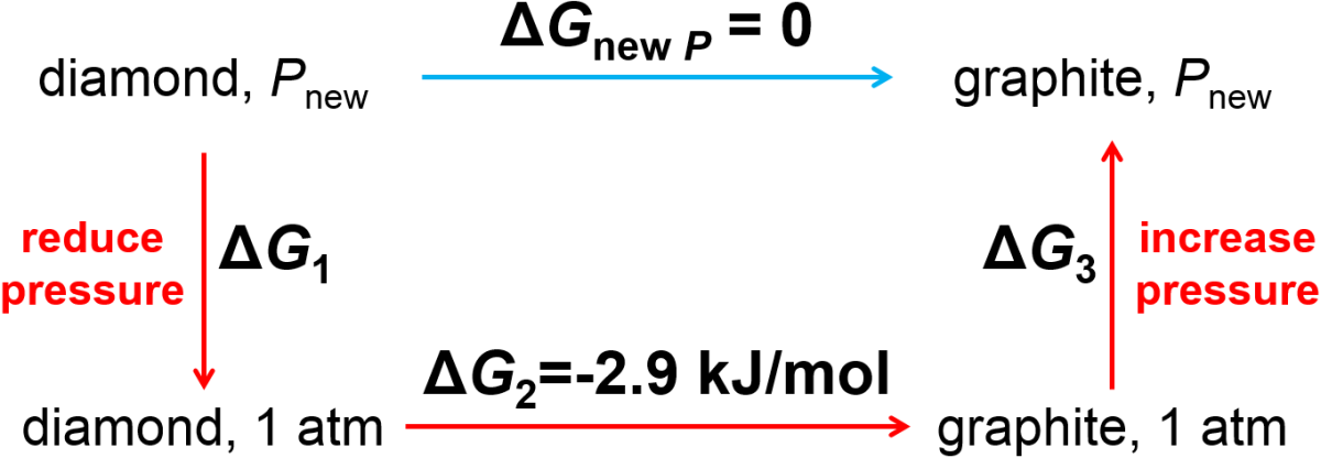
Fig. 4.1 Alternate path calculation to determine pressure at which the transition of diamond to graphite has a zero change in Gibbs free energy.
At a sufficiently elevated pressure (and assuming 298 K for all steps),
so that
Then we can calculate the Gibbs free energy change for the first and third steps using Eq. (4.8) to get
where \(\Delta P = P_\textrm{new} - P_\textrm{old}\).
We can combine the previous three equations
and define \(\Delta V = V_\textrm{gra} - V_\textrm{dia}\) to obtain
and then solve for \(\Delta P\) as
Note that we used molar volume here, or cubic meters per mole, which is merely the reciprocal of molar density (\(\rho\) in units of moles per cubic meter). We obtain the astonishingly high pressure of 15,000 atm as the pressure above which diamonds are thermodynamically stabler than graphite. In fact, researchers and some companies use this concept, together with optimized procedures, to make diamonds from graphite at very high pressure. Some companies use this to make small imperfect diamond crystallites for industrial purposes (e.g., abrasives) while others for synthetic gems that can be obtained at a fraction of the cost of non-synthetic diamonds, much to the chagrin of the diamond mining industry. There are even companies that specialize in converting human or pet remains into diamonds which is both amazing and creepy at the same time.
4.5. Phase Equilibrium
We frequently encounter solids, liquids, and gases in our everyday lives. In simple terms, molecules or atoms in a solid are bound together and possess a structural rigidity that tends to resists efforts to deform it, while molecules in a liquid are also bound together but are able to flow to conform to the shape of a container. In contrast, molecules of a gas are not bound to one another and instead expand to fill the available space. These are examples of states of matter. A closely related term is phase of matter which is a sample of matter that has uniform chemical and physical properties. Sometimes state and phase are used synonymously and it can get muddled. For instance, a container of liquid water with an ice cube in it contains two distinct phases and also two distinct states of matter. An example that nicely distinguishes the ideas would be to consider that oil and vinegar salad dressing at room temperature is in the liquid state but contains two phases with distinct densities and compositions. In this section we will consider the thermodynamic equilibrium between phases as there are deep connections between phase transitions and various thermodynamic variables.
4.5.1. Phase Diagram Review
Let’s first consider pressure vs temperature phase diagrams for water and carbon dioxide shown in Fig. 4.2. There is a lot of information to unpack in these. First off, the diagram indicates which state of matter is observed under equilibrium conditions as a function of pressure and temperature. These regions are separated from one another by so-called phase coexistence lines that indicate the set of points at which two phases can coexist.
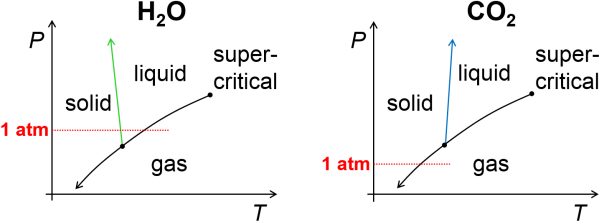
Fig. 4.2 Cartoon illustrations of pressure-temperature phase diagrams for water and carbon dioxide.
At high pressure and low temperature solids are typically observed. At low pressure and high temperature, gases are typically observed. In betwewen these conditions, liquids are typically observed but only at a sufficinetly high pressure. Specifically, notice that the two plots each have a point where the solid-liquid and liquid-gas coexistence lines interesect. This so-called triple point is the combination of pressure and temperature where solid, liquid, and gas can coexist in equilibrium as distinct phases. For water, we are accustomed to seeing the solid, liquid, and gaseous phases of water since its triple point pressure (~0.006 atm) is below our typical ambient pressure of ~1 atm. In contrast, the triple point of carbon dioxide is ~5 atm, or above our typical ambient pressure. For this reason, we are accustomed to observing dry ice (solid carbon dioxide) sublimate to gaseous carbon dioxide without first melting as is the case when we heat solid water.
At sufficiently high temperature and pressure there ceases to be a boundary between liquid and gas. The point at which this happens is called the critical point. When the pressure and temperature are both above the critical point, we observe a supercritical fluid which has some gas-like properties (e.g., molecules fill the available volume) and some liquid-like properties (e.g., an ability to dissolve some solutes). While we will devote little attention to the subject, supercritical fluids are important in a range of industrial processes including dry-cleaning, decaffeination, and power plants.
We will soon see that there is a deep quantitative connection between the thermodynamic properties of phase transitions and the slope of their coexistence lines, but for now let’s look at the connection more qualitatively. What should the sign of the slope be for the varoius coexistence lines? Let’s look at the solid gas coexistence line (below the triple point). In that case, if we took a sample of gas at a temperature below the triple point and subjected it to sufficiently high pressure we would convert the gas to a solid. At a temperature above the triple point (but below the critical point) if we subjected a gas to sufficiently high pressure it would convert to a liquid. These considerations lead us to expect that the slope of the solid-gas and liquid-gas coexistence lines on a pressure-temperature plot should each be positive. Now, what should the slope be for the solid-liquid coexistence line? It will depend on the relative density of the solid and liquid. In the more common case that the solid is more dense than the liquid, such as for carbon dioxide, we expect the slope to be positive. This would mean that if we subjeceted a sample of liquid carbon dioxide to sufficiently high pressure we would be able to generate solid carbon dioxide. On the other hand, ice is somewhat unusual since it has a lower density than liquid water (and floats, as a result), so we would expect the a sample of ice when subjected to sufficiently high pressure to convert to liquid water. This is reminiscent of the example problem for diamond and graphite where we saw that diamond is thermodynamically more stable than graphite at pressures above ~15,000 atm.
4.5.2. Clapeyron and Clausius-Clapeyron Equations
How does an increase in pressure imparct the equilibrium melting temperature or boiling temperature of a substance? An understanding of this will help us to partly map out the coexistence lines on a pressure-volume phase diagram. Since the coexistence line maps out the set of pressures and temperatures at which two phases are in equilibrium, we can set up a thermodynamic path as shown in Fig. 4.3 for the somewhat generic case of a phase transition between phases a and b. We will consider points \((P_1,T_1)\) and \((P_2,T_2)\) along the phase coexistence line where \(\Delta G = 0\) for the phase transition from a to b. Note that we are setting this up so that there is only a small, infinitesimal change in temperature and pressure between the two points (\(T_2 = T_1 + dT\) and \(P_2 = P_1 + dP\), where \(dT\) or \(dP\) may each be positive or negative so this is still quite general). With this set up, we can then use the differential of the Gibbs free energy (Eq. (4.6)) to add up changes around the thermodynamic path.
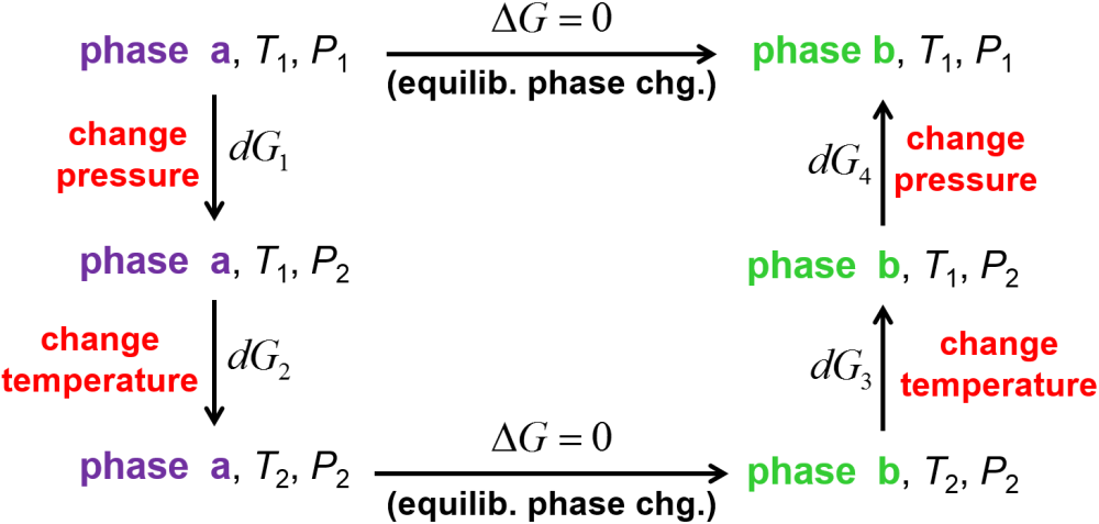
Fig. 4.3 Alternate path used to derive the Clapeyron equation.
All changes in Gibbs free energy add up to zero, and the vertical steps represented by \(dG_1\), \(dG_2\), \(dG_3\), and \(dG_4\) must also add up to zero.
For a pressure change of \(+dP\) in step 1 and \(-dP\) in step 4, we can use Eq. (4.6) to see that
Similarly, for temperature changes of \(+dT\) in step 2 and \(-dT\) in step 3, we can again use Eq. (4.6) to see that
Adding the four differential changes together for the non-zero steps 1-4, we get
so that
where the differences in entropy and volume upon the phase change from a to b are defined as \(\Delta S_\textrm{ph} = S_b - S_a\) and \(\Delta V_\textrm{ph} = V_b - V_a\). Next, we can remind ourself that for an equilibrium phase change at temperature \(T_\textrm{ph}\), the entropy change is \(\Delta S_\textrm{ph} = \frac{\Delta H_\textrm{ph}}{T_\textrm{ph}}\). From these, we arrive at a tidy little equation called the Clapeyron equation that relates the slope of the coexistence line \(\frac{dP}{dT}\) to thermodynamic quantities.
In the event that one of the two phases being considered is a gas (e.g., we are considering evaporation, sublimation, condensation, or deposition), we can actually get a more specific functional form that provides a more detailed (curved) shape of the coexistence line. To do this, we will first rearrange the Clapeyron equation (Eq. (4.10)) to obtain
When a condensed phase (solid or liquid) converts to a gas at constnat pressure, there is large increase in volume relative to the starting material such that we can approximate \(\Delta V = V_\textrm{gas} - V_\textrm{cond. phase} \approx V_\textrm{gas}\). Then, we can approximate the volume of the gas according to the ideal gas equation to get \(\Delta V = \frac{nRT}{P}\). For the purposes of this derivation, we are explicitly considering subplimation or evaporation so that we know the enthalpy change will be positive (\(\Delta H > 0\)). We can substitute this into the above equation to get
We will integrate both sides but need to first separate variables to get all the \(P\) terms with the \(dP\) and all the \(T\) terms with the \(dT\)
and we can integrate both sides with matched limits of integration and while assuming \(\Delta H\) to be approximately constant as a function of temperature and pressure
to get
which is known as the Clausius-Clapeyron equation. Now, with the Clapeyron and the Clausius-Clapeyron equations in hand, let’s practice using them with some example problems.
Example 6. What is the equilibrium melting temperature of ice at 1001 atm pressure? For water, \(\Delta H^\circ_\textrm{fus} = 6.0 \textrm{ kJ/mol}\) and \(V_\textrm{ice}-V_\textrm{water}=1.6\times10^{-6} \textrm{ m}^3\textrm{/mol}\). (Adapted from [17].)
We already know that water melts at equilibrium at 273 K and 1 atm and we are asked what melting temperature corresponds to 1001 atm, which corresponds to a pressure increase of 1000 atm, or \(\Delta P=1.01 \times 10^8 \textrm{ Pa}\). We can use the Clausius equation (Eq. (4.10)) to figure out the slope \(\frac{dP}{dT}\) from \(\frac{\Delta H_\textrm{fus}}{T\Delta V_\textrm{phases}}\) and we can then estimate that \(\frac{dP}{dT}=\frac{\Delta P}{\Delta T}\).
so that
From this we can conclude that
Since water has a negative slope for \(dP/dT\), we expect that an increase in pressure should correspond to a decrease in temeprature along the coexistence line and, indeed, that is what we calculated from the Clapeyron equation here.
Example 7. The boiling temperature of benzene at 1 atm is 353.2 K and the vapor pressure at 293 K is 10,000 Pa. What is the enthalpy of vaporization of benzene? (Adapted from [22].)
For this example, we are provided with two temperatures and two pressures, and from these we can use the Clausius-Clapeyron equation (Eq. (4.11)) to determine \(\Delta H_\textrm{vap}\). The Clausius-Clapeyron equation
can be rearranged to solve for \(\Delta H/n\) as
4.6. Maxwell Relations
We saw in Section 4.5 that there are deep connections between equilibrium and phase transitions and various quantities in thermodynamics. This is, in fact quite common, as there is overall a deep connectedness between many thermodynamic quantities. As you will soon see, it almost seems like everything in thermodynamics is a function of everything else. This can be unsettling at times, but it can also be really useful. Here we will introduce Maxwell relations with two main goals. First, we want to reveal some of the deep interrelatedness. Second, we want to obtain a tool to express difficult-to-measure quantities in terms of experimentally accessible quantities.
Maxwell relations come in two flavors. The first one shows how the variables \(P\), \(V\), \(T\), or \(S\) depend on the partial derivative of one of the four main ‘thermodynamic potentials’, namely \(U\), \(H\), \(A\), and \(G\). The second flavor shows some nifty connections between \(P\), \(V\), \(T\), and \(S\) using the magic of partial derivatives.
Here are the differentials of the four thermodynamic potentials. These were derived in Section 4.4.2 and Section 4.8.1.
From these, we can simply observe our first collection of Maxwell relations. For instance, we know that in the differential of internal energy, it must be the case that \((\partial U/\partial S)_V=T\) due to how we construct differentials. There are therefore eight of these equations, with two for each differential.
We can take the following a step further. Since we know that \(U\), \(H\), \(A\), and \(G\) are all state functions, it must be the case that the order of partial derivatives for each must commute due to Euler’s criterion for exactness. We can do this for each of the four state functions to obtain a new type of Maxwell relation. Let’s try one starting with internal energy.
Since internal energy is a state function, it must be true that the order of partial derivatives of \(V\) and \(S\) commute.
We saw above in Eq. (4.13) that \(\left( \frac{\partial U}{\partial S} \right)_V = T\) and \(\left( \frac{\partial U}{\partial V} \right)_S = -P\) so we can substitute both of these into Eq. (4.14) to obtain a new and less obvious relationship
Let’s try another one. Since enthalpy is a state function, it must be true that the order of partial derivatives of \(S\) and \(P\) commute.
We saw above in Eq. (4.13) that \(\left( \frac{\partial H}{\partial S} \right)_P = T\) and \(\left( \frac{\partial H}{\partial P} \right)_S = V\) so we can substitute both of these into Eq. (4.15) to obtain
The two remaining Maxwell relations obtained in this fashion are shown, below. Try deriving these yourself (or see problem Section 4.8.4).
Example 8. Use the equation of state for a van der Waals gas (Eq. (1.1)) to calculate \(\left( \frac{\partial U}{\partial V} \right)_T\) in terms of \(a\), \(n\), and \(V\). The goal here is to show you how Maxwell relations are potentially useful. In this case let’s say we need a more accurate equation of state than the ideal gas equation (\(PV=nRT\)) in order to optimize a gas phase chemical reaction. We can use the van der Waals gas equation of state together with some Maxwell relation analysis to obtain one of the van der Waals gas model parameters, as shown below.
Let’s start with the differential of internal energy
and then ‘complete the derivative’ by dividing all terms by \(dV\) and considering the situation at constant temperature.
We can substitute Maxwell relation \(\left( \dfrac{\partial S}{\partial V} \right)_T = \left( \dfrac{\partial P}{\partial T} \right)_V\) (obtained from the differential of the Helmholtz free energy) into the above equation to get
We can determine \(\left( \frac{\partial P}{\partial T} \right)_V\) by simply calculating the derivative of pressure from the vdW equation
and when the above is substituted into Eq. (4.16) provides
It is conceivable that one could measure the change in internal energy as a function of volume at constant temperature, or \(\left( \dfrac{\partial S}{\partial V} \right)_T\), and from this and knowledge of \(n\) and \(V\) obtain the value of the van der Waals \(a\) constant.
4.7. Summary of Key Equations
We introduced a whole lot of equations in this chapter! Let’s collect them all here for reference.
Equation |
Notes |
|---|---|
\(\Delta G = VdP - SdT\) |
Differential of Gibbs free energy (Eq. (4.6)) |
\(\Delta G_{T_2} \approx \Delta H_{T_1} - T_2 \Delta S_{T_1}\) |
Gibbs free energy change (approximation) for process at new temperature |
\(\Delta G_{\Delta T\textrm{ only}} = -S \Delta T\) |
Gibbs free energy change for temperature change only |
\(\Delta G_{\Delta P\textrm{ only}} = V \Delta P\) |
Gibbs free energy change for pressure change only |
\(\Delta G_{\Delta P \textrm{,gas}} = nRT \ln \dfrac{P_2}{P_1}\) |
Gibbs free energy change for gas change in pressure only |
\(\dfrac{dP}{dT} = \dfrac{\Delta S_\textrm{ph}}{\Delta V_\textrm{ph}}=\dfrac{\Delta H_\textrm{ph}}{T_\textrm{ph} \Delta V_\textrm{ph}}\) |
Clapeyron equation (Eq. (4.10)). Good for any phase transition. |
\(\ln \dfrac{P_2}{P_1} = -\dfrac{\Delta H_\textrm{ph}}{nR}\left( \dfrac{1}{T_2} - \dfrac{1}{T_1} \right)\) |
Clausius-Clapeyron equation (Eq. (4.11)). Only good for phase transitions involving a gas as one of the phases. |
\(\left( \dfrac{\partial U}{\partial S} \right)_V = \left( \dfrac{\partial H}{\partial S} \right)_P = T\) |
Maxwell relation (‘type 1’) |
\(\left( \dfrac{\partial U}{\partial V} \right)_S = \left( \dfrac{\partial A}{\partial V} \right)_T = -P\) |
Maxwell relation (‘type 1’) |
\(\left( \dfrac{\partial G}{\partial T} \right)_P = \left( \dfrac{\partial A}{\partial T} \right)_V = -S\) |
Maxwell relation (‘type 1’) |
\(\left( \dfrac{\partial G}{\partial P} \right)_T = \left( \dfrac{\partial H}{\partial P} \right)_S = V\) |
Maxwell relation (‘type 1’) |
\(\left( \dfrac{\partial T}{\partial V} \right)_S = -\left( \dfrac{\partial P}{\partial S} \right)_V\) |
Maxwell relation (‘type 2’) |
\(\left( \dfrac{\partial T}{\partial P} \right)_S = \left( \dfrac{\partial V}{\partial S} \right)_P\) |
Maxwell relation (‘type 2’) |
\(\left( \dfrac{\partial S}{\partial V} \right)_T = \left( \dfrac{\partial P}{\partial T} \right)_V\) |
Maxwell relation (‘type 2’) |
\(\left( \dfrac{\partial S}{\partial P} \right)_T = -\left( \dfrac{\partial V}{\partial T} \right)_P\) |
Maxwell relation (‘type 2’) |
4.8. Additional Problems
4.8.1. Differentials of Internal Energy and Enthalpy
What is the differential of internal energy in terms of \(T\), \(S\), \(P\), and \(V\)? What is it for enthalpy? Try deriving these using a similar procedure to the one used, above, for the Gibbs free energy.
Differentials of internal energy and enthalpy, SOLUTION
Answers:
For internal energy the differential form of the first law is
For a reversible path, the differential of work is \(dw = -PdV\) and the differential form of the second law differential is \(dS = dq/T\). We can substitute these into the above differential form of the first law to obtain the desired differential of internal energy.
Enthalpy is defined mathematically as \(H = U + PV\) so that \(\Delta H = \Delta U + \Delta(PV)\) and, using the first law, \(\Delta H = q + w + \Delta(PV)\). The differential of \(H\) is then
As with the internal energy, above, we can substitute \(dw = -PdV\) and \(dS = dq/T\) for a reversible path, and then obtain the desired differential of enthalpy.
4.8.2. Coexistence Line Slope
What would you expect the slope to be for a solid-liquid coexistence line on a pressure-temperature plot in the case where the density of the solid is equal to the density of the liquid?
Coexistence Line Slope, SOLUTION
Answer: The slope should be infinite. If the solid and liquid densities are the same then as pressure is increased, there is no ability to undergo a phase transition to a denser phase.
4.8.3. Free Energy Water Problems
Is the evaporation of water at 25 °C and 1 atm spontaneous, and if not, why is it typically true that water evaporates under these conditions?
Water has the somewhat uncommon property that the solid is less dense than the liquid. Without consulting tables, predict the sign of the slope \(dP/dT\) using the Clapeyron equation.
Free energy water problems, SOLUTION
Answers:
The evaporation of water at 373 K, 1 atm occurs at equilibrium, meaning
where \(\Delta H\) and \(\Delta S\) are both positive quantities. If we were to lower the temperature to 298 K, then we would find that \(\Delta G_{298\textrm{K}} > 0\). However, we also know from our every day experiences that water does indeed evaporate spontaneously at 298 K. This paradox can be resolved by considering the fact that water vapor, when it evaporates at 298 K, has a partial pressure that is lower than 1 atm. In fact, the reduction of pressure from 1 atm to the final partial pressure of water in the air will produce a net negative value of \(\Delta G\) that more than offsets the positive value of \(\Delta G_{298\textrm{K}}\) at 1 atm. If we considered the case in which the overall value of \(\Delta G_{298\textrm{K}}=0\) when factoring in the phase change and reduction in pressure and solved for the final pressure, we would obtain the vapor pressure of water. Lastly, note that water doesn’t always evaporate spontaneously at 298 K. Specifically, if the surrounding air were saturated with water vapor, meaning that the partial pressure of water in the air was equal to the vapor pressure of water at that temperature, then no net evaporation would occur. That would be like trying to dry yourself off in a sauna.
The Clapeyron equation states that
For freesing of liquid water, we expect a loss of entropy of the system, or \(\Delta S<0\), and an increase in volume of the system (since we know that ice floats in water), or \(\Delta V>0\). Based on these signs and the Clapeyron equation, it must be the case that \(\frac{dP}{dT}<0\) or that the slope of the solid-liquid coexistence line must be negative on a pressure-temperature plot. In contrast, for most substances like carbon dioxide where the density of the solid is greater than that of the liquid, we would expect \(\Delta V<0\) for freezing and, as before, \(\Delta S<0\), so that \(\frac{dP}{dT}>0\). Thus, by inspecting the Clapeyron equation and from the fact that \(\Delta S<0\) for freezing, one can determine whether the solid-liquid coexistence line has a positive or negative slope based simply on knowledge of the relative densities of the liquid and solid.
4.8.4. Maxwell Relation Derivation
You get one Maxwell relation for each of the thermodynamic potentials \(U\), \(H\), \(A\), and \(G\). The relations for \(U\) and \(H\) were derived in Section 4.6. Try deriving the two remaining Maxwell relations (for \(A\) and \(G\)) using Eq. (4.13) and a statement of exactness (partial derivatives commute for appropriate variables as seen from the corresponding differential in Eq. (4.12)).
Maxwell relations for \(A\) and \(G\), SOLUTION
Answers:
Since Helmholtz free energy \(A\) is a state function, it must be true that the order of partial derivatives of \(T\) and \(V\) commute.
We saw above in Eq. (4.13) that \(\left( \frac{\partial A}{\partial T} \right)_V = -S\) and \(\left( \frac{\partial A}{\partial V} \right)_T = -P\) so we can substitute both of these into Eq. (4.17) to obtain
Finally, since Gibbs free energy \(G\) is a state function, it must be true that the order of partial derivatives of \(P\) and \(T\) commute.
We saw above in Eq. (4.13) that \(\left( \frac{\partial G}{\partial T} \right)_P = -S\) and \(\left( \frac{\partial G}{\partial P} \right)_T = V\) so we can substitute both of these into Eq. (4.18) to obtain