7. Chemical Kinetics
Much of chemistry is concerned with transformations of one kind or another, whether for synthesis of therapeutics, enzyme-catalyzed metabolic processes within a cell, combustion of a fuel, etc. Chemical kinetics is the branch of physical chemistry that studies the rates of these transformations. It is important for answering practical questions of how long it takes a chemical process to occur or what conditions might yield a product most efficiently, and it is also a powerful tool for dissecting the mechanisms of complex chemical phenomena. There are some important connections between chemical kinetics and thermodynamics, but beyond this the two disciplines differ greatly in their basic approach. Thermodynamics is governed by a small number of deep, fundamental laws, while chemical kinetics is perhaps more a collection of phenomenological tools whose underlying mathematical framework of differential equations is applicable to a huge range of problems across science and engineering.
7.1. Stoichiometry and Kinetics
The concentrations of reagents in a chemical reaction all change together with rates that are proportional to their stoichiometric coefficients. Let’s take a look at how this works.
Consider the following, general, balanced chemical reaction
We know that as the reaction proceeds, products will increase and reactants will decrease, and the rates of these changes will occur with distinct ratios governed by the unitless stoichiometric coefficients \(\nu\). If the “extent of reaction” \(\xi\), in units of moles, is used to indicate the progress of the reaction, then we can write the number of moles \(n_i\) for the species \(i\) as a function of the initial number of moles of that species, \(n_{i,initial}\), \(\xi\), and \(\nu_i\). Since the stoichiometric coefficients \(\nu_i\) are defined as positive for products and negative for reactants, Eq. (7.1) can be used to succinctly describe formation of product or disappearance of reactant.
From there, we can calculate the rate of change of concentration \([i]\) for each species \(i\) as shown below. This assumes that the volume \(V\) is a constant as a function of time, which is a good assumption for many reactions that are relatively dilute.
The variable \(R\), introduced above, is the rate of reaction and it is the same for all species. It is sometimes also called the intensive rate of the reaction. Note from the following how the rate of reaction \(R\) compensates for the stoichiometric coefficients.
practice calculating reaction rates
Question: \(\require{mhchem}\ce{CO2}\) Consider the reaction \(\ce{3H2 + N2 -> 2NH3}\). If the concentration of ammonia is increasing by 3.5 mM/second, what is the (intensive) rate of the reaction, \(R\)? What are the rates of change of the concentration of \(\ce{H2}\) and \(\ce{N2}\), including the correct sign?
Answers:
\(\triangleright\;\) \(R=(1/2) \times \textrm{d}\ce{[NH3]}/\textrm{d}t=1.75 \textrm{ mM/s}.\)
\(\triangleright\;\) \(\textrm{d}\ce{[N2]}/\textrm{d}t=(-1)\times R = -1.75 \textrm{ mM/s}.\)
\(\triangleright\;\) \(\textrm{d}\ce{[H_2]}/\textrm{d}t=(-3)\times R = -5.25 \textrm{ mM/s}.\)
7.2. Rate law expression
Experimentally, we see that the rate of a reaction \(R\) can have different dependences on the concentrations of each of the reactants. If a rate of a reaction is linearly proportional to the amount of a given reactant, it is called first order with respect to the reactant. There can also be zeroth order, second order, higher orders, fractional orders, and even negative orders. Sometimes people also mention the overall order of the reaction which is the sum of the individual orders (provided none are negative). For the moment, we won’t ask why a reaction is a certain order and we will simply treat it as experimentally determined. The Rate Law Expression contains information about order for each reagent in the reaction, although the reaction orders are not generally the stoichiometric coefficients. Finally, the units of the rate constant are variable and depend on the overall order of the reaction.
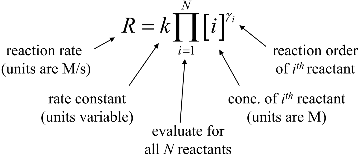
Fig. 7.1 Rate law expression and its terms.
practice writing rate law
Question: For the reaction \(\ce{NO + 1/2O2 -> NO2}\), the reaction orders are \(\gamma_\ce{NO}=2\) and \(\gamma_{\textrm{O}_2}=1\). Write out a rate law expression showing the correct exponents. What are the units of the rate constant \(k\)?
Answers:
\(\triangleright\;\) \(R=k[\ce{NO}]^2[\ce{O2}]\)
\(\triangleright\;\) \(\; k\) has units of \(1/(\textrm{M}^2\textrm{s})\) so that \(R\) has the correct units of \(\textrm{M/s}\).
How is the reaction order determined? Let’s review two methods. First is the method of initial rates where the initial rate is measured for several different concentrations of reactants. A second approach, called the method of isolation, uses a series of kinetic measurements, one for each reactant in limiting amounts, in order to compare the concentration vs time data to signatures of first order, second order, etc.
Method of initial rates. For each reagent in a reaction, measure the rate of the reaction while varying only that reactant’s concentration. The rate law expression predicts how much the reaction rate will change as a function of concentration of a reactant for a given reaction order, and we can use that dependence to determine the reaction order for each reactant. Let’s write that out generically for reagent \(\ce{[A]}\).
and
We can divide the above two expressions and then take the natural log to get the reaction order for \(\textrm{[A]}\).
Isolation method. Use a large excess of all but one reagent and then observe the decay of that reagent with respect to time. In this case, “a large excess” means that the dependence on that reagent goes to zeroth order, such that the reagent may be omitted from the rate law expression and is roughly constant. We will see soon that zeroth-order, first-order, and second-order reactions exhibit different signatures. With knowledge of those signatures, it is then possible to study the rate dependence on concentration of the isolated species in order to figure out its reaction order. This will make more sense after we look at the integrated rate laws. But for now, let’s think about the isolation method a little more concretely. Consider the reaction \(\ce{A + B -> C}\) with \(R=k\ce{[A]}^\alpha \ce{[B]}^\beta\). When \(\ce{[A]}\) is in large excess, its concentration will be approximately constant as a function of time so we can rewrite the rate law expression as \(R=k’\ce{[B]}^\beta\). Similarly, when \(\ce{[B]}\) is in large excess, we can write \(R=k''\ce{[A]}^\alpha\).
practice finding reaction order
Questions: Use the data, below, to determine the order of the reaction with respect to each of \(\textrm{A}\) and \(\textrm{B}\) for the reaction \(\ce{A + B -> C}\). What is the value of \(k\), including its units? Use the isolation method.
\(\textrm{[A] (M)}\) |
\(\textrm{[B] (M)}\) |
initial rate \(R \; \textrm{(M/sec)}\) |
|---|---|---|
\(3.3 \times 10^{-4}\) |
\(2.1 \times 10{-2}\) |
\(0.10\) |
\(3.3 \times 10^{-4}\) |
\(7.8 \times 10{-2}\) |
\(0.38\) |
\(4.7 \times 10^{-4}\) |
\(7.8 \times 10{-2}\) |
\(0.78\) |
Answers:
Note:
Here is potentially useful shortcut you should know for some simple problems. If the concentration of one species is doubled (and the others are held constant) and this doubles \(R\), you get \(2^1=2\) or \(\gamma=1\). Or if one concentration is doubled (and the others are held constant) and this quadruples \(R\), you get \(2^2=4\) or \(\gamma=2\). However, if one concentration goes up 12% and \(R\) goes up 18.5% you might not easily intuit that \(\gamma=3/2\). Because of this, it is good to know the more general logarithm approach shown here.
7.3. Integrated Rate Laws
Let’s do some classic kinetics problems of different orders to build up a toolkit for solving these types of problems. We will restrict ourselves to an important subset of exactly solvable examples that are all relatively common and that for the most part don’t require any differential equation solutions methods beyond separation of variables. Our starting point will be be to combine the rate law expression with the definition of the (intensive) rate of the reaction, as shown, below.
After this, our method will generally use the following steps. As you read through the kinetics problems, below, try to follow where you are in these four steps, and make sure the math makes sense for each step. There are also some general notes, below, that we will use as we solve various reaction classes in the sections that follow.
Evaluate the combined rate law / rate of reaction expression shown above.
Separate variables.
Integrate both sides.
Solve for the concentration(s) of interest as a function of time.
Notes on implementing the above steps for various reactions. You will get to practice these for a number of examples, shortly.
If there are multiple parallel reactions for a given species, the total rate of change for a species is the sum of rates for the individual reactions in which it appears. This matters for reactions like the following.
\(\textrm{A} \rightarrow \textrm{B}\) in parallel with \(\textrm{A} \rightarrow \textrm{C}\)
\(\textrm{A} \rightleftharpoons \textrm{B}\)
\(\textrm{A} \rightarrow \textrm{B} \rightarrow \textrm{C}\)
Sometimes you may need to relate an unknown species to a known species.
For the parallel reactions \(\textrm{A} \rightarrow \textrm{B}\) and \(\textrm{A} \rightarrow \textrm{C}\), use the solution for \([\textrm{A}(t)]\) to solve for \([\textrm{B}(t)]\) or \([\textrm{C}(t)]\).
For \(\textrm{A} \rightleftharpoons \textrm{B}\), use \([\textrm{A}(t)]+[\textrm{B}(t)] = [\textrm{A}(t_0)] + [\textrm{B}(t_0)]\) to put \([\textrm{B}(t)]\) in terms of \([\textrm{A}(t)]\).
For the sequential reactions \(\textrm{A} \rightarrow \textrm{B} \rightarrow \textrm{C}\), use \([\textrm{A}(t)]\) to solve for \([\textrm{B}(t)]\) and \([\textrm{B}(t)]\) to solve for \([\textrm{C}(t)]\).
Notes on interpreting your results once you have them. Calculating the time-dependent concentration of a species of interest isn’t the end of the story. It takes a little more work to get key quantities of interest. You may want to find the time when a concentration has reached half (or some arbitrary fraction of) the original concentration, or when the concentration of an intermediate is maximum, or to determine the equilibrium constant
To find the half-life \(t_{1/2}\) of species \(\textrm{X}\), solve for the value of \(t_{1/2}\) when \([\textrm{X}(t_{1/2})]=[\textrm{X}(0)]/2\). You could use the same approach to find the tenth-life where \([\textrm{X}(t_{1/10})]=[\textrm{X}(0)]/10\) or some other fraction.
To find the time where the concentration of intermediate species \(\textrm{S}\) is maximum, differentiate \([\textrm{S}(t)]\) with respect to time and set equal to zero. That is, use \(\textrm{d}[\textrm{S}(t)]/\textrm{d}t=0\) and \(t=t_\textrm{max}\) just like you would for any function.
Equilibrium will occur when \(t\) approaches infinity. E.g., you can use \([\textrm{A}_\textrm{eq}]=[\textrm{A}(\infty)]\).
Be careful with your stoichiometry!
It is equally valid to balance a reaction as \(\textrm{A}\rightarrow\textrm{B}\) or as \(2\textrm{A}\rightarrow2\textrm{B}\). In thermodynamics, this requires a little care to indicate clearly that, for instance, the change in enthalpy refers to the reaction as written or per mole of one reagent, etc. In kinetics, we must also exercise similar care. Let’s take a look at what happens to the value of the intensive rate and rate constant depending on how reaction is balanced.
For the first-order reaction written as \(\textrm{A}\rightarrow\textrm{B}\), the combined rate law / rate of reaction expression equation gives us
wheras for case #2, the first-order reaction is written as \(2\textrm{A}\rightarrow2\textrm{B}\), the combined rate law / rate of reaction expression equation gives us
Hopefully you can see that the intensive rate \(R_1\) for case #1 is twice that of the intensive rate \(R_2\) and that the kinetic rate constant for case #1 is half that of case #2. In this case, the intensive rate and rate constants perfectly compensate to give the same overall eventual expression for \([\textrm{A}(t)]\) (see Section 7.3.2).
The simplest solution to this problem may be to balancing chemical reactions with the smallest integer coefficients possible, but in any event keep an eye out for this potential source of confusion.
7.3.1. 0th order, A \(\rightarrow\) B
Zeroth order reactions are not particularly common, but one important example is an enzyme-catalyzed reaction with an excess of the enzyme’s substrate. Assume that the reaction \(\textrm{A} \rightarrow \textrm{B}\) is zeroth order with respect to \(\textrm{A}\).
Evaluating the combined rate law / rate of reaction expression
gives us the following.
From here we can separate variables
and then integrate both sides
to get
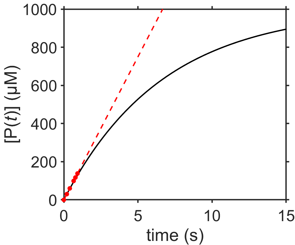
Interpret results. Since the rate of change of the reaction doesn’t change with respect to time, the rate continues to decrease from the initial concentration \([\textrm{A}(0)]\) with a constant rate and so we observe a linear decrease. Does the reaction keep going in a straight line forever? No, obviously that won’t work since at sufficiently long times we would then observe a negative concentration for \([\textrm{A}(t)]\) and the concentration of \([\textrm{A}(t)]\) would increase indefinitely. Eventually, the reaction would slow down and plateau. Was our mathematical result wrong? Mostly no. We essentially assumed that substrate would stay a constant concentration which is not true at sufficiently long times.
Fig. 7.2 Plot of \([\textrm{A}(t)]\) and \([\textrm{B}(t)]\) for \(\textrm{A}\rightarrow\textrm{B}\), zeroth-order integrated rate law with \(k=0.2\;\textrm{M/s}\). The dashed lines indicate that after \(t=5\;\textrm{s}\) the results are meaningless since \([\textrm{A}(t)]<0\) and \([\textrm{B}(t)]>1\;\textrm{M}\). source
practice zeroth order kinetics
Questions: Look at the (simulated) data plotted, below, for the balanced enzyme-catalyzed reaction where substrate goes to product, \([\textrm{S}]\rightarrow[\textrm{P}]\), that is zeroth order with respect to \([\textrm{S}]\) at early times and that has \([\textrm{P}(t_0)]=0\).
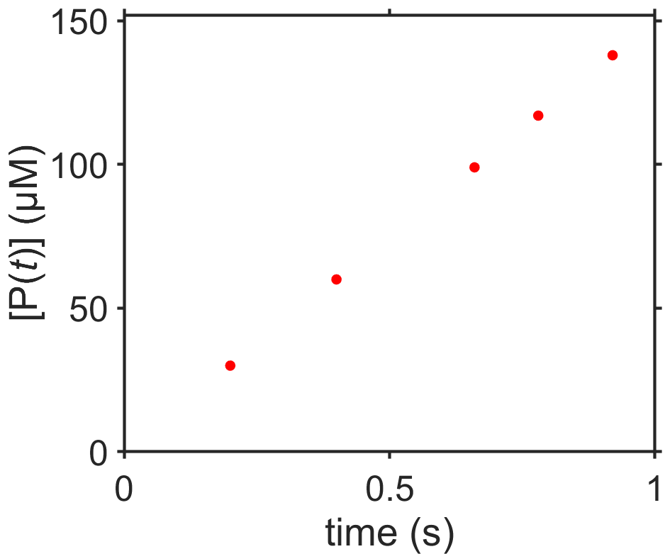
Fig. 7.3 Zeroth-order kinetics for the reaction \(\textrm{S}\rightarrow\textrm{P}\).
source
If \([\textrm{P}(0)]=0\), can you write a generic expression for \([\textrm{P}(t)]\)?
Estimate the value of the rate constant \(k\) including correct units.
Make a sketch of \([\textrm{P}(t)]\) as \(t\) goes to very long times.
Answers:
We just saw in Section 7.3.5 that for a zeroth order reaction, the reactant concentration decreases linearly. Here, this means substrate S decreases according to \([\textrm{S}(t)] = [\textrm{S}(0)] - kt\). Since product P is initially zero, we know that the sum of substrate and product concentrations at all times must equal the initial substrate concentration, or \([\textrm{S}(0)]=[\textrm{S}(t)]+[\textrm{P}(t)]\). From combining these two equations we can see that \([\textrm{P}(t)]=kt\).
We can calculate the slope of the line from the \([\textrm{P}(t)]\) vs \(t\) plot to determine \(k\) in our solution \([\textrm{P}(t)]=kt\). We get \(k = \textrm{d}[\textrm{P}]/\textrm{d}t \approx \Delta\textrm{P}/\Delta t\) where if we estimate from the plot we get \(k = 150 \times 10^{-6} \textrm{ M}/1 \textrm{s} = 1.5 \times 10^{-4} \textrm{M/s}\).
The product can’t keep increasing forever and must eventually plateau. This is illustrated in the plot, below, together with the original data at early times.
7.3.2. 1st order, A \(\rightarrow\) B
Let’s assume \(\textrm{A} \rightarrow \textrm{B}\) is now first order with respect to \(\textrm{A}\), meaning \(\gamma_\textrm{A}=1\). We will see that this produces an exponentially decaying concentration as a function of time. Exponential decays are ubiquitous in nature and we will see that they have the important property that the time to decay by a given fraction of the current amount is a constant regardless of how much the sample has already decayed. The most well-known example of an exponential decay is probably radioactive decay, which is characterized by its half-life, or characteristic time to decay by 50%.
Evaluating the combined rate law / rate of reaction expression for \(\textrm{A} \rightarrow \textrm{B}\), first-order
gives us the following.
From here we can separate variables
and integrate both sides
to get
Since all concentrations will be positive, we can drop the absolute terms. Then we can exponentiate both sides and rearrange to get
We see that the rate of change of \([\textrm{A}(t)]\) decreases as a function of time and that the shape of the function is an exponential decay that approaches zero at long times (see Fig. 7.5).
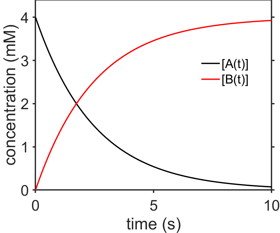
Fig. 7.5 Plot of integrated rate law for \([\textrm{A}(t)]\) for \(\textrm{A}\rightarrow\textrm{B}\), first-order, assuming \(t_0=0\). source
The half-life \(t_{1/2}\) is time at which the concentration is half its original amount. Somewhat uniquely, the half-life for first-order decay is independent of concentration. This is unlike the case for zeroth order decay where we saw that the half-life decreased over time.
or
practice first-order kinetics
Questions: Data are plotted, below, for the radioactive decay of technetium in the contrast agent Sestamibi as part of a “MIBI scan” of a patient’s heart. Use the data to answer the following questions. To keep things simple, you may simply refer to the reactant as \([\textrm{A}]\) and the product as \([\textrm{B}]\).
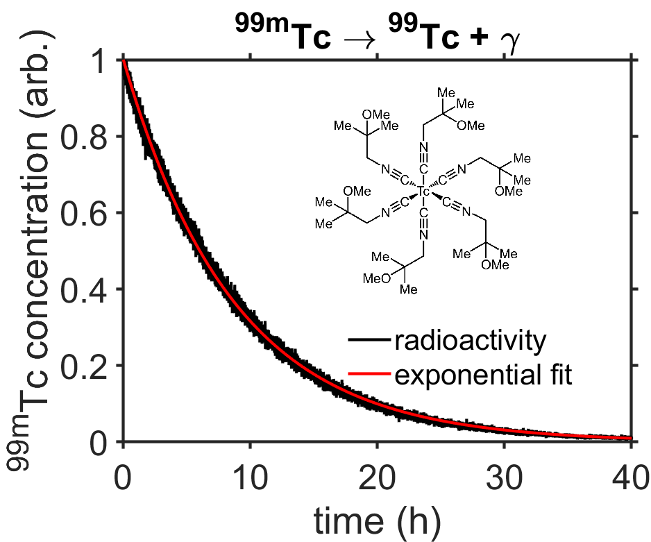
Fig. 7.6 Radioactive decay of technetium-99m. The concentration of technetium-99m is proportional to radioactivity measured by a Geiger counter. (Data from [4].) source
What is the rate constant \(k\) for the radioactive decay including correct units?
What is the \(1/5^\textrm{th}\) life of technetium-99m?
Answers:
Estimate the half-life by examining the plot, to get \(t_{1/2}\approx6\;\textrm{h}\). From this use the equation \(k=\ln(2)/t_{1/2}\) to calculate \(k=0.12/\textrm{h}\).
You could read \(t_{1/5}\) from the plot, but let’s instead calculate \(t_{1/5}\) using our knowledge of \(k\) from problem 1, above. In that case we have \([\textrm{A}(t_{1/5})]=[\textrm{A}(0)]/5=e^{-k(t_{1/5})}\), which we can use to solve for \(t_{1/5}\) as \(t_{1/5}=\ln(5)/k=14.6\;\textrm{h}\).
We can solve for \([\textrm{B}(t)]\) using
while also substituting our answer for \([\textrm{A}(t)]\) to get
7.3.3. All non-1st order, A \(\rightarrow\) B
Rather than keep marching through the orders, let’s solve the reaction \(\textrm{A} \rightarrow \textrm{B}\) for all reaction orders besides first-order (whose integration is different from the other orders). While we will derive the general result here, we will focus on the second order reaction kinetics to find expressions for \([\textrm{A}(t)]\), half-life, and to examine the decay behavior.
Evaluating the combined rate law / rate of reaction expression for \(\textrm{A} \rightarrow \textrm{B}\) of order \(\gamma\neq 1\)
gives us the following.
From here we can separate variables
and integrate both sides
to get
We can rearrange to get the following general solution for all orders of \(\gamma\neq 1\).
For the case of \(\gamma=2\) (a second-order reaction) this becomes
We can also calculate the half-life using
which we can solve for \(t_{1/2}\) as
Let’s think about these results. In Fig. 7.7 I plotted first and second order decays. Both start at a concentration of 1 M (units omitted on y-axis). For first order, k=0.2/s and for second order k=0.2/(M*s). The first order reaction decays more quickly, although both approach zero at long times. The decays also have different shapes. I marked the half, quarter, and eighth concentrations with black circles or squares. Can you see that the half-life of the second order decay becomes longer and longer (5 s, 10 s, 20 s) while the half-life of the first order decay stays constant (~3.5 s)? This is an important finding. The half-life of an exponential decay doesn’t depend on the starting concentration while that of a second order gets longer and longer as the concentration decreases. In contrast, recall that a zeroth-order decay has a half-life that decreases during the decay.
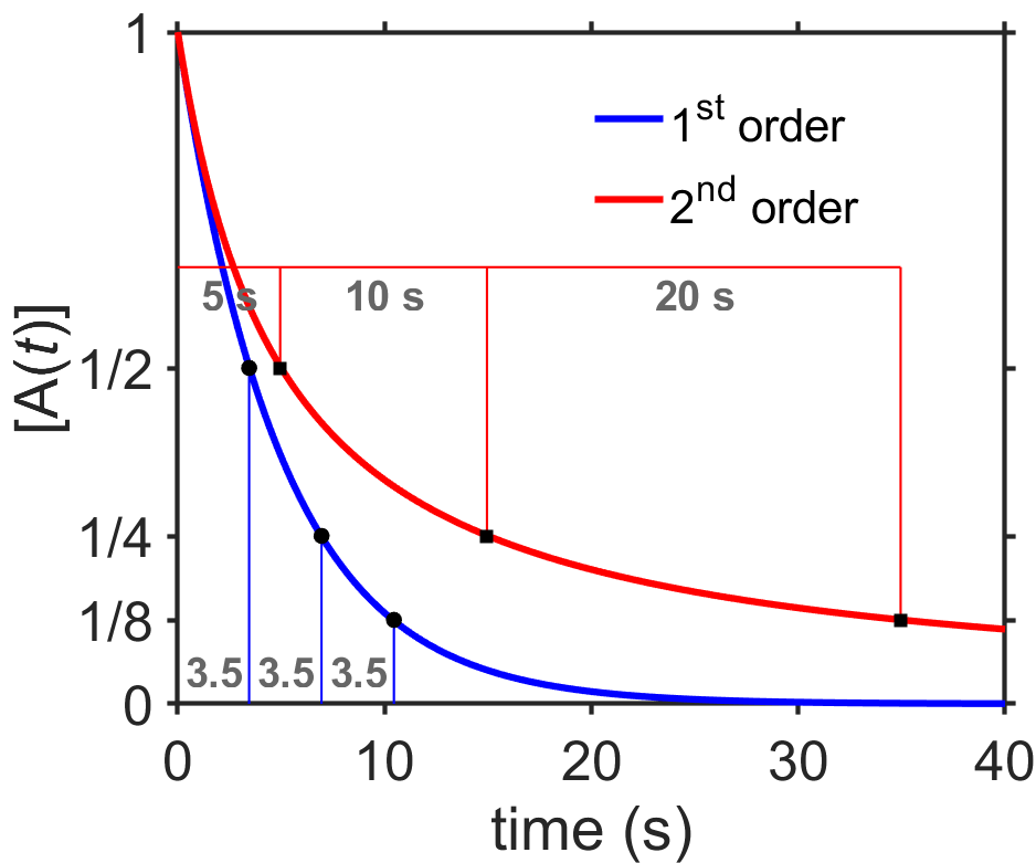
Fig. 7.7 Comparison of \([\textrm{A}(t)]\) with \(\textrm{A}\rightarrow\textrm{B}\) for first- and second-order reactions. Successive half-lives for the first-order reaction are constant while those of the second-order reaction increase. source
practice kinetics with order > 1
Questions: Consider the third-order reaction \(\textrm{A}\rightarrow\textrm{B}\).
What are the units for the rate constant, \(k\)?
What is \([\textrm{A}(t)]\) for the third-order reaction \(\textrm{A}\rightarrow\textrm{B}\)?
What is the time required to reach 10% of the initial concentration?
Answers:
\({1/(\textrm{sM}^2)}\)
\([\textrm{A}(t)] = 1/\sqrt{1/[\textrm{A}(t_0)]^2 + 2k(t-t_0)}\)
\(t_{1/10}=99/(2k[\textrm{A}(t_0)]^2)\)
7.3.4. Parallel, A \(\xrightarrow{k_1}\) B, A \(\xrightarrow{k_2}\) C
Chemical reactions often happen in parallel. Let’s consider the case where reactant \(\textrm{A}\) can convert into product \(\textrm{B}\) or product \(\textrm{C}\), which can be written as the set of parallel chemical reactions \(\textrm{A} \rightarrow \textrm{B}\) and \(\textrm{A} \rightarrow \textrm{C}\). In principle, the pathways could be of the same or different orders as each other, however, we will focus on the case where all reactions are first-order with respect to \(\textrm{A}\) but with different rate constants, \(k_{\textrm{1}}\) and \(k_{\textrm{2}}\). We will solve \([\textrm{A}(t)]\), \([\textrm{B}(t)]\), and \([\textrm{C}(t)]\), together with the half-life of \(\textrm{A}\).
Before we dive into the math, though, it may be uesful to think of a physical analogy for our two parallel reactions. Imagine a bucket with two holes (Fig. 7.8). The rate of water leaking out of the bucket depends on the size of the hole, with bigger holes passing more water and vice versa. As the water in the bucket drains out, the pressure decreases and the water flows out more slowly from each of the holes. The size of each hole may be thought of analogously to the rate constant, where a larger hole corresponds to a larger rate constant and vice versa.

Fig. 7.8 Leaky bucket analogy for parallel first-order reactions \(\textrm{A} \xrightarrow{k_1} \textrm{B}\) and \(\textrm{A} \xrightarrow{k_2} \textrm{C}\) with \(k_1<k_2\).
In terms of setting up our overall differential equation will be that the rate of change of \([\textrm{A}(t)]\) results from the sum of the rate of changes along each of the two pathways, according to
What if there were three or more parallel reactions? You could add them all up similar to the above step.
Next, for each of the separate reactions \(\textrm{A} \rightarrow \textrm{B}\) and \(\textrm{A} \rightarrow \textrm{C}\), evaluate the combined rate law / rate of reaction expressions.
and
We can rearrange and substitute these into the overall differential equation, giving
If we used \(k_{\textrm{total}}=k_1+k_2\) we will simply have the same form of the first-order decay differential equation Section 7.3.2 which gives us the same solutions for exponential decay and half-life. Here we will assume that \(t_0=0\).
and
Next, let’s take a look at how to calculate \([\textrm{B}(t)]\). To do this, we will go back to the combined rate law / rate of reaction expression, now for \(B\).
We can plug in our solution for \([\textrm{A}(t)]\) to the right side of the above equation
then separate variables
and integrate both sides
which gives
and if we evaluate the right hand side and assume \([\textrm{B}(t_0)]=0\) then we get the following equation for an exponential plateau
We could use the same approach to calculate \([\textrm{C}(t)]\).
Interpret results. We saw that \([\textrm{A}(t)]\) has the form of a first-order reaction with an exponential decay to zero using an overall rate constant that is the sum of the individual rate constsants \(k_\textrm{total}=k_1+k_2\). For \([\textrm{B}(t)]\) and \([\textrm{C}(t)]\) the term \((1-e^{-k_\textrm{total}t})\) says there will be an exponential plateau as \(t\rightarrow\infty\). The constants \([\textrm{A}(0)]k_1/k_\textrm{total}\) in \([\textrm{B}(t)]\) tell us the maximum concentration of \([\textrm{B}(t)]\) will be the fraction \(k_1/k_\textrm{total}\) of \([\textrm{A}(0)]\) (assuming that \([\textrm{B}(0)]=0\)). Similarly, \([\textrm{C}(t)]\) also has an exponential plateau and reaches the maximum value of \([\textrm{A}(t_0)]k_2/k_\textrm{total}\). Lastly, the ratio \([\textrm{B}(t)]/[\textrm{C}(t)]=k_1/k_2\).
practice parallel reactions
Questions: Consider the following scenarios with parallel reactions.
For three parallel first-order chemical reactions, \(\textrm{A} \xrightarrow{k_1} \textrm{B}\), \(\textrm{A} \xrightarrow{k_2} \textrm{C}\), and \(\textrm{A} \xrightarrow{k_3} \textrm{D}\), what are \([\textrm{A}(t)]\), \([\textrm{B}(t)]\), \([\textrm{C}(t)]\), and \([\textrm{D}(t)]\)? Assume that \([\textrm{B}(0)]=[\textrm{C}(0)]=[\textrm{D}(0)]=0\).
For two parallel second-order chemical reactions, \(\textrm{A} \xrightarrow{k_1} \textrm{B}\) and \(\textrm{A} \xrightarrow{k_2} \textrm{C}\), what are \([\textrm{A}(t)]\), \([\textrm{B}(t)]\), and \([\textrm{C}(t)]\)? Assume that \([\textrm{B}(0)]=[\textrm{C}(0)]=0\).
Answers:
Three parallel first-order reactions have a solution that is nearly identical to the case we derived in this section with two parallel first-order reactions except that \(k_\textrm{total}=k_1+k_2+k_3\).
\[[\textrm{A}(t)] = [\textrm{A}(t_0)]e^{-k_\textrm{total}t}\]\[[\textrm{B}(t)] = [\textrm{A}(t_0)]\frac{k_1}{k_\textrm{total}}(1 - e^{-k_\textrm{total}t})\]\[[\textrm{C}(t)] = [\textrm{A}(t_0)]\frac{k_2}{k_\textrm{total}}(1 - e^{-k_\textrm{total}t})\]\[[\textrm{D}(t)] = [\textrm{A}(t_0)]\frac{k_3}{k_\textrm{total}}(1 - e^{-k_\textrm{total}t})\]
For two parallel second-order chemical reactions, we can adapt our two parallel first-order reaction derivation, above. Here, \(k_\textrm{total}=k_1+k_2\).
\[\left(\frac{\textrm{d}[\textrm{A}(t)]}{\textrm{d}t} \right)_{\textrm{total}} = k_1[\textrm{A}(t)] + k_2[\textrm{A}(t)] = -(k_1+k_2)[\textrm{A}(t)]^2\]The equation above can be solved for \([\textrm{A}(t)]\) as to give a solution like we calculated for a single second-order reaction, above, in Section 7.3.3 to get.
\[[\textrm{A}(t)] = \frac{1}{1/[\textrm{A}(t_0)] + k_\textrm{total}(t-t_0)}\]To solve for \([\textrm{B}(t)]\) we need to do a little more work. We can write out the combined rate law / rate of reaction for the reaction \(\textrm{A} \rightarrow \textrm{B}\) to get
\[\frac{1}{+1}\frac{\textrm{d}[\textrm{B}(t)]}{\textrm{d}t} = k_1[\textrm{A}(t)]^2\]We can substitute in our solution for \([\textrm{A}(t)]\) from above, separate variables, and set up the integrals shown below.
\[\int\limits_{0}^{[\textrm{B}(t)]}\textrm{d}[\textrm{B}(t)] = k_1\int\limits_{0}^{t}\frac{\textrm{d}t}{\left(1/[\textrm{A}(t_0)]+k_\textrm{total}t\right)^2}\]Solving the integral gives us the following expression for \([\textrm{B}(t)]\)
\[[\textrm{B}(t)] = \frac{k_1}{k_\textrm{total}}\left([\textrm{A}(0)] - \frac{1}{1/[\textrm{A}(0)]-k_\textrm{total}t}\right)\]which we can adapt to solve for \([\textrm{C}(t)]\)
\[[\textrm{C}(t)] = \frac{k_2}{k_\textrm{total}}\left([\textrm{A}(0)] - \frac{1}{1/[\textrm{A}(0)]-k_\textrm{total}t}\right)\]
7.3.5. Bidirectional, A \(\require{mhchem}\ce{<=>[k_1][k_2]}\) B
The bidirectional reaction \([\textrm{A}]\rightarrow[\textrm{B}]\) is a particularly important problem since it allows us to make an important connection between kinetics and thermodynamics via the equilibrium that is established at long times. We will treat this as a series of parallel reactions that go in opposite directions between \(\textrm{A}\) and \(\textrm{B}\).
As with the parallel first order reactions studied in Section 7.3.4, we will start by writing out the overall rate of change of \([\textrm{A}(t)]\) sum of the rate of changes along each of the two pathways, with the difference that now one of the reactions is positive and the other is negative.
As in Section 7.3.4, for each of the separate reactions \(\textrm{A} \rightarrow \textrm{B}\) and \(\textrm{B} \rightarrow \textrm{A}\), we will evaluate the combined rate law / rate of reaction expression. Note that the signs are opposite, as expected, since the forward reaction depletes \(\textrm{A}\) while the reverse reaction resupplies it.
and
We can rearrange and substitute these into the overall differential equation, giving
We can put \([\textrm{B}(t)]\) in terms of \([\textrm{A}(t)]\) by urecognizing that the total amount of \(\textrm{A}\) and \(\textrm{B}\) is constant at all times, namely
so that
Plugging in the above expression for \([\textrm{B}(t)]\) into the overall differential equation gives
In principle, we could separate and integrate the above equation, but there are a lot of terms and it would be easy to get confused during the integration. Instead, we will take a closer look at the differential equation to recognize the meaning of some of those constants. This will help us to simplify the equation and will later help us with our interpretation.
Let’s consider what happens to the differential equation at \(t\rightarrow\infty\) once the system has equilibrated to \([\textrm{A}_\textrm{eq}]\) and \([\textrm{B}_\textrm{eq}]\) and there is no further net change to the system. In that case
and we can solve for \([\textrm{A}_\textrm{eq}]\)
Looking at the differential equation, now, we can factor out the term \(-(k_1+k_2)\) to get
Now we can see that the last term in the differnetial equation is just \([\textrm{A}]\), giving us an equation that looks much easier to work with.
Next we can separate variables
and integrate both sides
to get
Finally, we can exponentiate both sides
to get the solution
We can also take a quick peek at the value of the equilibrium constant for this reaction. The easiest way to do this is to go back to the equilibrium state
and we can rearrange to see that \(k_1[\textrm{A}_\textrm{eq}] = k_2[ \textrm{B}_\textrm{eq}]\)
so that the equilibrium constant
Interpret results. At time \(t=0\), we can see that \([\textrm{A}(0]=[\textrm{A}_0]\) and at long times the system will relax to equilibrium. It reaches the same equilibrium state regardless of the value of \([\textrm{A}(0)]\), in agreement with our thermodynamics-based understanding of the equilibrium state. How does this happen mathematically? We can see that if \([\textrm{A}(0)]>[\textrm{A}_\textrm{eq}]\) then the sytem will undergo an exponential decay down to the equilibrium concentration and if \([\textrm{A}(0)]<[\textrm{A}_\textrm{eq}]\) then the system will undergo an exponential plateau up to the equilibrium concentration. The rate of the exponential decay is the sum of the rates \(k_1+k_2\) so equilibrium will be reached more quickly when either one of the rate constants is increased.
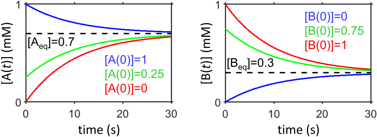
Fig. 7.9 Bidirectional first-order kinetics showing \([\textrm{A}(t)]\) and \([\textrm{B}(t)]\) for three different initial conditions that always relax to the same equilibrium state (each condition is shown in a different color).
practice bidirectional first-order reaction
Questions: Consider the bidirectional first-order reaction \(\textrm{A}\rightleftharpoons\textrm{B}\) that is first-order with respect to both \(\textrm{A}\) and \(\textrm{B}\).
Write an expression for the value of \([\textrm{B}_\textrm{eq}]\) in terms of \(k_1\), \(k_2\), \([\textrm{A}(0)]\) and \([\textrm{B}(0)]\).
Examine the data in Fig. 7.9. What is the equilibrium constant? What is the sum of the decay constants that dictates the exponential decay/plateau? What are the individual constants \(k_1\), \(k_2\)?
Answers:
Rather than doing a bunch of work to derive this result from scratch, let’s just notice the symmetry of the reaction \(\textrm{A}\rightleftharpoons\textrm{B}\) and then adjust our equation for \([\textrm{A}_\textrm{eq}]\), above by swapping instances of \(\textrm{A}\) and \(\textrm{B}\) along with swapping instances of \(k_1\) with \(k_2\) to get
The equilibrium constant is given by \(K=[\textrm{B}_\textrm{eq}]/[\textrm{A}_\textrm{eq}]=0.3/0.7=0.43\). The exponential term \(e^{-(k_1+k_2)t}\) provides either an exponential decay or plateau to the equilibrium value and the half-life of that decay or plateau can be used to calculate the sum of the decay constants \(k_1+k_2\) for any of the three conditions shown. From the condition with \([\textrm{B}(0)]=1\;\textrm{mM}\), the system decays decays half way to the equilibrium concentration (i.e., from \(1\;\textrm{mM}\) to \(0.65\;\textrm{mM}\), in \(t_{1/2}\approx7\;\textrm{s}\), indicating that \(k_1+k_2=\ln(2)/t_{1/2}\approx0.1/\textrm{s}\). We can use the above information to solve for \(k_1\) and \(k_2\) by using the equations \(k_1+k_2=0.1/\textrm{s}\) and \(K=k_2/k_1=0.43\) to obtain \(k_1=0.233/\textrm{s}\) and \(k_2=0.1/\textrm{s}\).
7.3.6. Bimolecular A+B \(\rightarrow\) C
Bimolecular reactions of the form \(\ce{A + B -> C}\) that are first-order with respect to each reagent are relatively common in chemistry and biology. Evaluating the combined rate law expression Eq. (7.2) gives us
To solve this, we will use an extent of reaction strategy that keeps track of how much of the concentration of each species has changed as a function of time, similar to how we kept track of the number of moles of each species in Eq. (7.1). Here, for the \(i^{th}\) species we get
where \(\nu_i\) is the stoichiometric coefficient of the \(i^{th}\) species and \([x(t)]\) is a variable in units of \(\textrm{M}\) that accounts for changes in the concentration of each chemical species. We can apply Eq. (7.3) to each species in our combined rate law expression to get
and
We can substitute all of these into our combined rate law expression, above, to get
With all the brackets and such, it is kind of hard to look at the above equation. Here it is, rewritten in a more informal, but readable way.
We can separate variables and set up our integrals to get
The right-hand side integral of Eq. (7.4) is just \(kt\). The left-hand side integral takes more work but is not too hard to solve if you use an algebra trick for fractions.
where
Now, the left-hand side integral of Eq. (7.4) becomes
which is easy to solve
We will explicitly assume here that all quantities within the absolute value terms are positive so we can drop the absolute value symbols. Now, we can combine our separate solutions to the left-hand side and right-hand side integrals in Eq. (7.4) to get
We can clean up the above expression and solve for \(x\). Once we have \(x\) then we can determine \(\ce{[A($t$)]}\), \(\ce{[B($t$)]}\), and \(\ce{[C($t$)]}\).
Combining some of the natural logarithm terms gives us
We can exponentiate both sides and rearrange to get
which can be solved for \(x\) to give
The above equation for \(x\) can be substituted into the following equations as \([x(t)]\) to determine the concentrations of each of the three species.
After that heavy lifting, let’s take a look at an example (Fig. 7.10). In the example, \(\ce{[B($0$)]>[A($0$)]}\) and at long times, \(\textrm{A}\) is completely consumed, \(\ce{[C($\infty$)]}=\ce{[A($0$)]}\), and \(\ce{[B($\infty$)]}=\ce{[B($0$)]}-\ce{[A($0$)]}\), as expected.
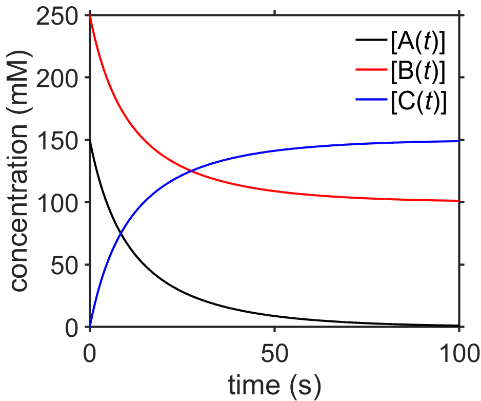
Fig. 7.10 Plot of integrated rate law for the bimolecular addition reaction \(\ce{A + B -> C}\) with \(k=0.4\;\textrm{1/Ms}\) source
practice calculating half-life for bimolecular reaction
Question: Calculate the half-life of the bimolecular addition reaction \(\ce{A + B -> C}\), assuming that \(\ce{[A($t$)]<[B($t$)]}\).
Answer: The half-life should depend on the rate constant \(k\) as well as the initial concentration of \(\ce{[B{$_0$}]}\). We can solve for that by finding the time at which \(x\) reaches half of its maximum value, where its maximum value will be the same as \(\textrm{A}_0\) since at long times all of \(\textrm{A}\) is converted into \(\textrm{C}\).
We can solve the above equation for \(t_{1/2}\) to get
For the values used in our example (Fig. 7.10), we would predict that \(\textrm{A}\) would have a half-life of ~8.4 s, as in agreement with the plot.
What about the situation when \(\ce{[A($0$)]}=\ce{[B($0$)]}\)? Isn’t that just the second-order reaction as described in Section 7.3.3? Yes! One can obtain the second-order result by taking the limit of the above result as \(\ce{[A($0$)]}\rightarrow\ce{[B($0$)]}\) using L’hopital’s rule (give it a try!).
7.3.7. Bimolecular bidirectional, A+B \(\rightleftharpoons\) C
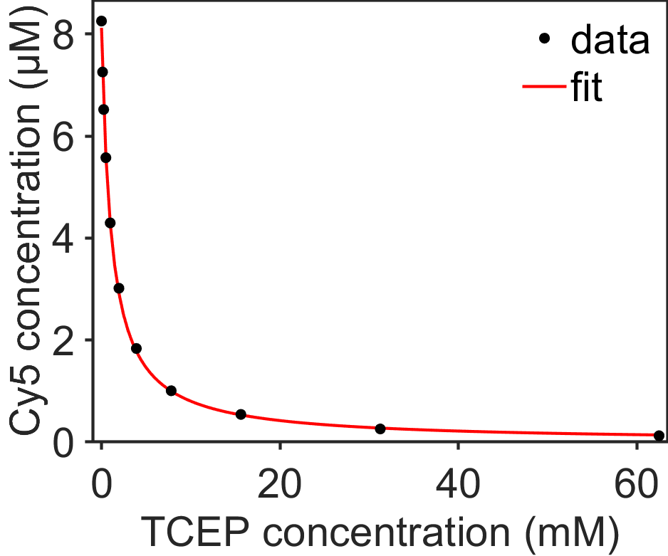
Bimolecular reactions of the form \(\ce{A + B <=> C}\) that are first-order with respect to each reagent are also relatively common in chemistry and biology. However, the exact solution is cumbersome. Here we will only consider a subset of problems for which \([\textrm{A}(0)]<<[\textrm{B}(0)]\), which means that the more abundant reagent (\(\textrm{B}\), here) has an approximately constant concentration at all points during the reaction and will have no time dependence. The reaction is said to be pseudo-zeroth order with respect to \(\textrm{B}\) but still first-order with respect to \(\textrm{A}\).
We can write the rate-law expression for the forward reaction as
This reduces the problem to the bidirectional first-order reaction \(\textrm{A}\rightleftharpoons\textrm{C}\) with the forward rate constant \(k_1^*\) and the reverse rate constant \(k_2\), which we solved above in Section 7.3.5. Putting \(k_1[\textrm{B}]\) in place of \(k_1\) into our result for \([\textrm{A}(t)]\) from Section 7.3.5 gives
and
The above two equations both show that the rate of decay and \([\textrm{A}_\textrm{eq}]\) are both dependent on \([\textrm{B}]\).
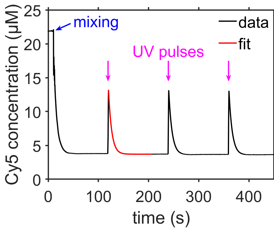
Fig. 7.11 Plot showing quenching of the dye Cy5 by 4 mM TCEP (tris(2-carboxyethyl)phosphine) due to reversible formation of an adduct via reaction \(\ce{[Cy5] + [TCEP] <=> [Cy5-TCEP]}\). Brief ultraviolet pulses could dissociate the Cy5-TCEP adduct. The data are fit well by a decaying exponential of the form shown in Eq. (7.5). The reversible switching of Cy5 with TCEP can be used for super-resolution fluorescence microscopy as described in [5]. source
Lastly, we can show how \([\textrm{A}_\textrm{eq}]\) relates to the association constant \(K_\textrm{a}\), where \(K_\textrm{a}=k_1/k_2\) and is the reciprocal of the concentration of \([\textrm{B}]\) where \([\textrm{A}]\) is 50% bound, that is when \([\textrm{A}]=[\textrm{A}(0)]/2\).
7.3.8. Sequential, A \(\xrightarrow{k_1}\) B \(\xrightarrow{k_2}\) C
Sequential first-order reactions of the form \(\textrm{A} \xrightarrow{k_1} \textrm{B} \xrightarrow{k_2} \textrm{C}\) are common in biology. Among other interesting things, they allow the formation of transient intermediates, and tuning of the rate constants can allow control of the time when the intermediate is maximized together with the peak concentration of the maximum. We will assume that \([\textrm{B}(0)]=[\textrm{C}(0)]=0\). Also, we will initially consider the case where \(k_1\neq k_2\), but we will go back for the case of equal rate constants.
Our first step is to solve the first-order reaction \(\textrm{A} \xrightarrow{k_1} \textrm{B}\) with rate constant \(k_1\), which we already calculated in Section 7.3.2. Assuming that \(t_0=0\), that expression becomes
Next, we will work on solving for the concentration of \(\textrm{B}\) as a function of time. We have two reactions involving \(\textrm{B}\) and, as before, we will set this up using the fact the rate of change of \(\textrm{B}\) is the sum of the rates of changes of each of the two reactions.
We have now combined the rate law expression and rate of reaction for many reactions in the preceding sections. Doing so here gives us that
and
We can combine these to get the total differential equation that we will be solving.
This equation is a bit trickier to solve. So far, we have been using separation of variables to get concentration terms on the left side of the equation and time terms on the right side of the equation so that we can integrate both sides. Unfortunately, that won’t work here since we now have the sum of a time term and a concentration term and we can’t do the separation.
To get through this, we will use a TRICK called an integrating factor that can help with some differential equations. First, we will move the \(k_2[\textrm{B}]\) term to the left side of the equation.
This doesn’t properly separate variables, but we at least have the two concentration terms containing \([\textrm{B}(t)]\) on the same side of the equation. The next step is the key part. We will multiply both sides of the above equation by a function \(f\) that is carefully chosen to simplify the two terms of the left hand side to one term by using the product rule backwards. Specifically, we want to find an integrating factor (function) \(f\) that we can use to multiply both sides of the above equation and that also converts the two terms from the left hand side into a single term.
Let’s multiply both sides of the equation by \(f\)
and then impose the condition on \(f\) that it can (hopefully) enable two terms to be combined
Next, we can expand the right hand side of the above equation using the product rule
and then cancel common terms in the resulting equation
to get
After canceling out the \([\textrm{B}(t)]\) terms and separating variables we get the following differential equation
whose solution is
Ok, we did a bunch of work to figure out that our integrating factor is \(f=e^{k_2t}\) which allows us to write the following, now as a single term:
When we combine the integrating factor with the right side of the equation we are trying to solve, we get
Now we can combine these new left and right hand sides that have been multipled by \(f\)
We will treat the new quantity \([\textrm{B}(t)]e^{k_2t}\) here as one integrating variable and time as the other when we separate variables
Next, integrate both sides
which gives
and then we get the solution for the intermediate \([\textrm{B}(t)]\)
Next we will use the expression for \([\textrm{B}(t)]\) to solve for \([\textrm{C}(t)]\). The combined rate law / rate of reaction expression for \(\textrm{C}\) is
and substituting in our solution for \([\textrm{B}(t)]\) gives
We can easily separate variables for the above this time
which, after some algebra, gives us the solution
Summary of results for the sequential first order reaction \(\textrm{A}\xrightarrow{k_1}\textrm{B}\xrightarrow{k_2}\textrm{C}\) with \(k_1 \neq k_2\).
Interpret results. You can see from the above three equations showing the integrated rate laws and from Fig. 7.13 that \([\textrm{A}(t)]\) is simply an exponential decay, \([\textrm{B}(t)]\) peaks at some early time before decaying to zero, and \([\textrm{C}(t)]\) rises and plateaus to the same concentration as \([\textrm{A}(0)]\). What would you predict would happen if \(k_2\) became larger or smaller? It is worthwhile to play with these equations a bit in a program that can plot them for you (MATLAB, Microsoft Excel, etc.) so that you can gain an intuition for interplay between the two rate constants.
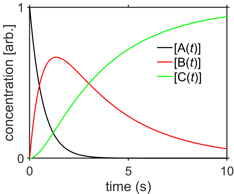
Fig. 7.13 Concentrations of species for the sequential first-order reactions \(\textrm{A}\xrightarrow{k_1}\textrm{B}\xrightarrow{k_2}\textrm{C}\) for \(k_1=1.5/\textrm{s}\) and \(k_2=0.3/\textrm{s}\). source
Wait…what happens if both rate constants are the same (\(k_1=k_2=k\))? The expressions for \([\textrm{B}]\) and \([\textrm{C}(t)]\) both contain a denominator with \(k_2-k_1\) that looks like it would go to infinity, but this can’t be true. In fact, if we go back to the integrals where we solved for \([\textrm{B}(t)]\) and \([\textrm{C}(t)]\) we can solve for this case separately as shown below..
At the integral step
if we have \(k_1=k_2=k\) then we get
which we can integrate
to get
so that
Next we can determine \([\textrm{C}(t)]\). Our combined rate law / rate of reaction expression for \([\textrm{C}(t)]\), including a substitution for \([\textrm{B}(t)]\) from above, is
We can separate variables
and then integrate
to get
Just for fun… what if we had the situation where there were a series of \(n\) first-order chemical reactions with identical rate constants? Let’s take a look.
The reaction scheme we are considering is of the form
We already solved for the first two states \([\textrm{A}_1]\) and \([\textrm{A}_2]\), in the two step reaction scheme, as
and
To move forward, we can basically continue our recursive procedure where one solution is fed into the differential equation that is used to calculate the next solution. Let’s look at a couple of these and then show the general equation.
We can use \([\textrm{A}_2(t)]\) to calculate \([\textrm{A}_3(t)]\). We do this by writing out the combined rate law reaction rate equation for \([\textrm{A}_3(t)]\) as shown below. This has already combined both reactions that impact the concentration of \([\textrm{A}_3(t)]\) (coming in from \([\textrm{A}_2(t)]\) and going out to \([\textrm{A}_4(t)]\)).
Next we can subsitute in our solution for \([\textrm{A}_2(t)]\) to get
then add \(k[\textrm{A}_3(t)]\) to both sides to get
and then use the integrating factor \(e^{kt}\) to get to the separable differential equation
that, once separated, is
and can be integrated to give
If you think about the procedure a little bit, you can hopefully see that each subsequent reaction adds a factor of \(kt/(n-1)\)
As a brief aside, note that the above function for \([\textrm{A}_n(t)]\) is essentially the Gamma probability distribution
Lastly, we can calculate the concentration of the final state \([\textrm{A}_{n+1}(t)]\) using its combined rate law / rate of reaction expression
We can separate the integral and solve using integration by parts using the following recursive relationship, but it is tedious for large \(n\).
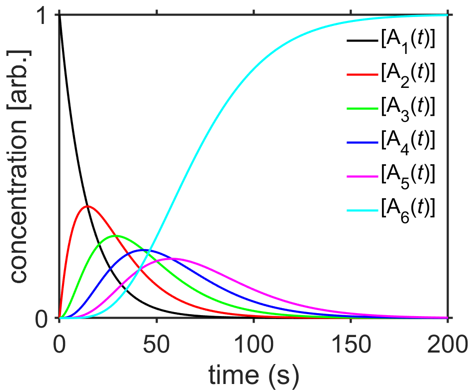
Fig. 7.14 Integrated rate law solution for the sequential reactions \(\ce{A1 ->[k] A2 ->[k] A3} \cdots \ce{A$_n$ ->[k] A$_{n+1}$}\) with \(n=5\) and \(k=0.0693/\textrm{sec}\). source
7.3.9. Integrated rate laws final thoughts
This section (Section 7.3) elaborated in some detail several classic and important classes of reactions in chemical kinetics and much intuition can be gained from these. Some can be adapted relatively straightforwardly.
For instance, what if you want to find the integrated rate law for the second-order reaction \(2\textrm{A}\rightarrow\textrm{B}\) which differs from the \(\textrm{A}\rightarrow\textrm{B}\) reaction considered in Section 7.3.3? In that case, revisiting the combined rate law / rate of reaction expression shows that it will be a simple variation on the second order result from Section 7.3.3. Here the combined rate law / rate of reaction expression is
and this can be rearranged to give
and as the same overall effect of using \(2k\), now, in place of the second-order result for \(\textrm{A}\rightarrow\textrm{B}\) derived in Section 7.3.3
Summary of Integrated Rate Law Results
zeroth-order |
\([\textrm{A}(t)] = [\textrm{A}(t_0)] - k(t-t_0)\) |
first-order |
\([\textrm{A}(t)] = [\textrm{A}(t_0)] e^{-k(t-t_0)}\) |
second-order |
\([\textrm{A}(t)] = \dfrac{1}{1/[\textrm{A}(t_0)] + k(t-t_0)}\) |
all non-first order |
\([\textrm{A}(t)]^{\gamma-1} = \dfrac{1}{1/[\textrm{A}(t_0)]^{\gamma - 1} + k(t-t_0)(\gamma-1)}\) |
Bimolecular |
\(\ce{[A($t$)]$=$[A($0$)]}-[x(t)]\) |
parallel first-order |
\([\textrm{A}(t)] = [\textrm{A}(t_0)]e^{-(k_1+k_2)(t-t_0)}\) |
bidirectional first-order |
\([\textrm{A}(t)] = [\textrm{A}_\textrm{eq}] + \left([\textrm{A}(0)] - [\textrm{A}_\textrm{eq}]\right)e^{-(k_1 + k_2)(t-t_0)}\) |
sequential first-order |
\([\textrm{A}(t)] = [\textrm{A}(0)]e^{-k_1 t}\) |
7.4. Temperature Dependence
Chemical reactions are in general sensitive to temperature, with most reactions occuring more quickly at a higher temperature. This temperature dependence, which is familiar even to nonscientists through experiences in the kitchen and elsewhere, was a subject of great interest in the mid-1800s and beyond [6][7].
Maxwell showed that gas molecules have a well-defined distribution of kinetic energies, where the fraction above a given energy \(E\) is proportional to \(\exp[-E/RT]\). This led to work from Pfaundler, van’t Hoff, and Arrhenius who considered the case of a gas-phase reaction at chemical equilibrium. In that scenario, the equilibrium constant would be equal to the ratio of the forward and reverse rate consants. Because the equilibrium constant itself had a dependence on temperature, given by the van’t Hoff equation
it was believed that the forward and reverse constants would also have a similar temperature dependence. For the hypothetical equilibrium reaction it was proposed that the forward and reverse reactions were each in equilibrium with an activated form of a molecule most closely analogous to the modern idea of the transition state. These ideas are summarized in the Arrhenius equation that predicts the temperature-dependence of a rate constant
where \(A\) is the pre-exponential factor, \(E_\textrm{a}\) is the activation energy, \(R\) is the gas constant, and \(T\) is temperature.
In its most common form, the two Arrhenius equation parmaters \(A\) and \(E_\textrm{a}\) have no temperature dependence. The pre-exponential factor \(A\) has overall units that match the rate constant. It always includes a \(1/\textrm{s}\) term, however, and it is sometimes described as being proportional to the rate of collisions or number of attempted reactions per second. Of the colliding molecules, only the fraction of molecules whose kinetic energy is larger than \(E_\textrm{a}\) are able to react, where this fraction of activated is proportional to \(\exp[-E_\textrm{a}/RT]\).
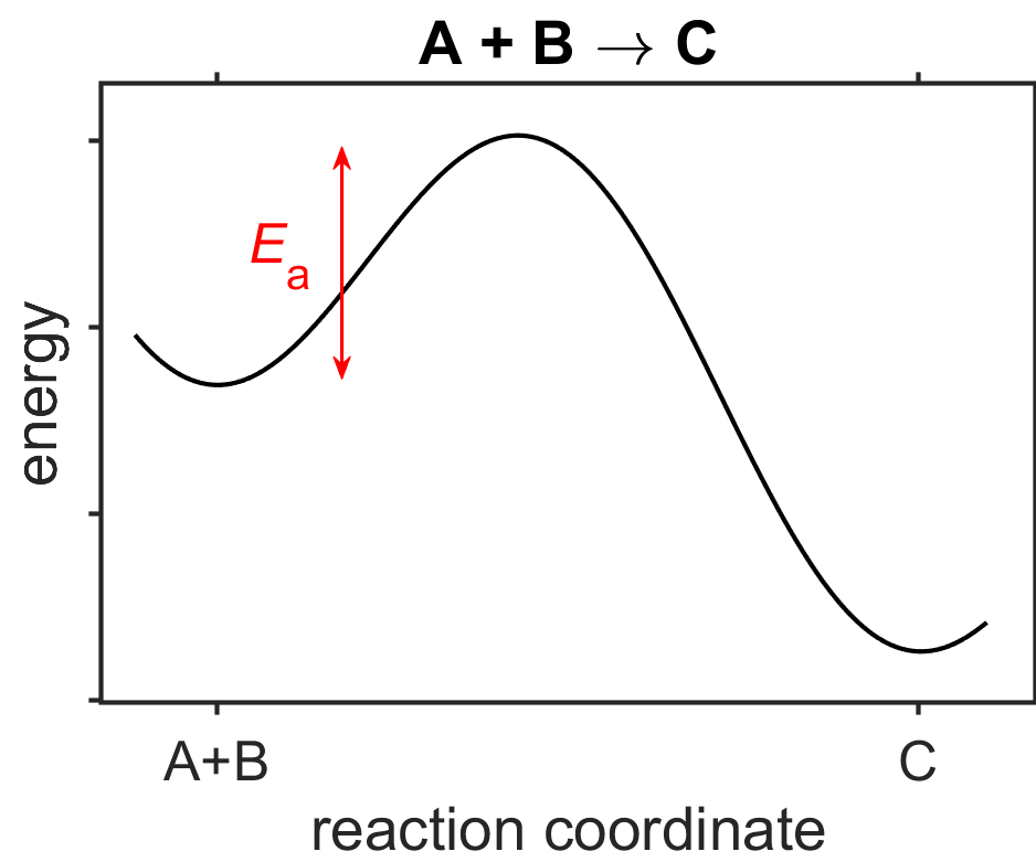
Fig. 7.15 Energy vs reaction coordinate plot for the hypothetical reaction \(\textrm{A}+\textrm{B}\rightarrow\textrm{C}\). source
Although the Arrhenius equation is a largely empirical relationship, it has been widely used for the past century due to its fairly good agreement with experiment and its relatively simple and intuitive form. As we will see later, the Arrhenius equation can also help explain some key aspects of catalysis as we will see in section Section 7.5.
practice temperature-dependence of kinetic rate constant
Question: Using a high-pressure tube, Radzicka and Wolfenden [8] measured the kinetics of hydrolysis of glycylglycine to glycine, \(\ce{GG + H2O -> 2G}\), at temperatures between ~100 °C and 200 °C (two points are shown in the table, below). From these measurements, we can estimate the half-life for hydrolysis of a peptide bond at normal physiological temperatures.
What are values of the Arrhenius prefactor \(A\) and activation energy \(E_\textrm{a}\) for the hydrolysis of glycylglycine?
Estimate the half-life of the peptide bond in glycylglycine at approximately physiological temperature (37 °C). Note that the reaction is first-order with respect to glycylglycine.
\(T\;(\textrm{K})\)
\(k\;(\textrm{s}^{-1})\)
\(392\)
\(10^{-6}\)
\(464\)
\(10^{-4}\)
Answers:
Let’s solve \(E_\textrm{a}\) by writing out the Arrhenius equation for each of the two conditions and then dividing the two expressions to eliminate \(A\).
This can be solved for \(E_\textrm{a}\) to give
We can substitute \(E_\textrm{a}\) back into one of the Arrhenius expressions to solve for \(A\) as
In order to estimate the half-life of the glycylglycine peptide bond, let’s first calculate the rate constant at 298 K, using our values for \(A\), \(E_\textrm{a}\), and the gas constant \(R=8.31\;\textrm{J/K mol}\).
From the value of \(k_{298\textrm{K}}\) and our knowledge of first-order kinetics (Section 7.3.2), we can calculate the expected half-life using
Radzicka and Wolfenden used more data points and some additional analysis, but reported \(E_a=96.1\;\textrm{kJ/mol}\) and \(t_{1/2}=~350\;\textrm{years}\) which are not far from our values. The ~300 year hydrolysis half-life of an amide bond (at neutral pH, 25 °C) is a good benchmark value to remember for a biochemist.
Limitations of the Arrhenius model. The Arrhenius equation is a simple and useful model that gives us intuition about the physical basis of the temperature dependence of reaction rates. In more advanced models such as collision theory or transition state theory (each of which are also known by other names) it is shown that the prefactor is actually dependent on temperature. The prefactor \(A\) in these cases would typically contain a term \(aT\) or \(aT^{1/2}\), although the exponential term generally has a stronger temperature dependence.
7.5. Catalysis
Catalysts are substances that speed up chemical reactions but are not consumed during the reaction. They can be organic or inorganic molecules, solids, proteins, RNA molecules, etc., and small amounts of catalyst are often able to strongly impact the rate of a chemical reaction. All areas of chemistry are impacted by catalysts in some form, from the industrial processes (e.g., synthesis of ammonia for fertilizer), to catalytic converters that help automobiles burn fuel more cleanly, to chlorofluorocarbon pollutants that can catalyze the destruction of ozone within the stratosphere. Catalysts are also essential in biology, where uncatalyzed biochemical reactions are generally slow, but catalysts enable organisms to efficiently direct chemical processes to optimize their fitness.
Consider the decomposition of a solution of hydrogen peroxide. At approximately neutral pH and ~300 °C, it spontaneously decomposes at a relatively low rate (i.e., the hydrogen peroxide solution is stable in your medicine cabinet), however, in the presence of catalysts like \(\mathrm{HBr}\) or the enzyme catalase, hydrogen peroxide can decompose \(~10^4\) to \(~10^{15}\) times faster, respectively.
The Arrhenius model for temperature-dependence of chemical reactions (Section 7.4) can provide some insight into how catalysts speed up chemical reactions. In the Arrhenius equation, \(k=A\exp[-E_\textrm{a}/RT]\), either the pre-exponential factor or the exponential term could be increased by a catalyst, the largest increases occur in the pre-exponential factor as a result of the lowering of the activation energy \(E_\textrm{a}\) along the catalyzed reaction pathway. Notably, the lower activation energy increases both the the forward and reverse reaction rates, but does not alter the energies of the reactants and products or their equilibrium state (Fig. 7.16).
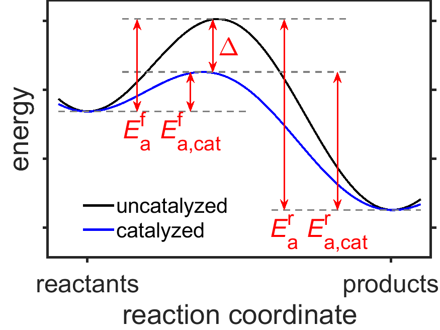
Fig. 7.16 Energy vs reaction coordinate plot for a hypothetical reaction in the presence and absence of a catalyst. The catalyst does not change the energies of reactant or product but lowers the energy barriers for the forward and reverse reactions (\(E_\textrm{a,cat}^\textrm{f}\) and \(E_\textrm{a,cat}^\textrm{r}\), respectively) by the amount \(\Delta\). source
Let’s take a look how the Arrhenius equation shows us that a catalyst impacts the rates of both the forward and reverse reactions without impacting the position of the equilbrium. As can be seen in Fig. 7.16, reducing the height of the energy barrier by the amount \(\Delta\) reduces both the forward and reverse activation energies by the same amount. If we write out the Arrhenius equation for the forward and reverse rate constants, \(k_\textrm{f}\) and \(k_\textrm{r}\), respectively, we get
and
If we assume that \(A^f\) and \(A^r\) are the same with or without the catalyst, we can see that the ratio of the rate constants is unchanged by the presence of the catalyst according to
which reveals that the forward and reverse rates are increased by the same factor of \(\exp[\Delta/RT]\). We saw in Section 7.3.5 that the equilibrium constant for a reversible reaction contains the ratio of the forward and reverse rate constants, which are unchanged, here, by the presence of the catalyst. From a thermodynamic perspective, since the energies of the reactants and products are unchanged by the presence of the catalyst, one would expect the position of the equilbirium to be unchanged by the presence of the catalyst given the equilibrium relationship \(\Delta G^\circ=-RT\ln(K)\).
7.6. Diffusion-Limited Reactions
Reactions that involve diffusion face a “speed limit” resulting, for instance, from the time it takes for two molecules to find each other. In solution, which is our concern here, reacting molecules will diffuse separately but may occasionally associate with one another for a period in what is called an ‘encounter’ (Fig. 7.17).
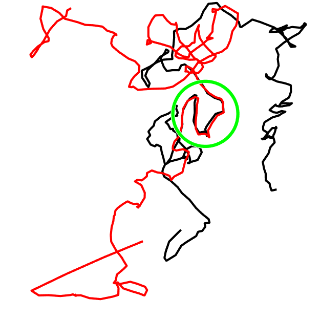
Fig. 7.17 Cartoon illustration of two diffusing molecules in solution that diffuse together for a short period of time called an encounter (green circle). source
During an encounter, the solvent around the two molecules temporarily confines the two molecules to share a relatively small volume, and there may be a burst of collisions between the two molecules, where each collision has some chance of leading to product. As a result, the collisions tend to be clustered within an encounter (Fig. 7.18).
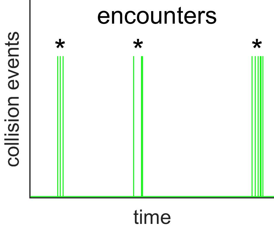
Fig. 7.18 Cartoon illustration of multiple encounters, where several collisions occur during each encounter. source
Let’s consider the model bimolecular association reaction \(\ce{A + B -> P}\). We can imagine that as moleclues \(\ce{A}\) and \(\ce{B}\) diffuse in solution, they will form encounter pairs \(\ce{\{AB\}}\) with a rate that depends on their concentrations and their rates of diffusion. (We use the funny braces around \(\ce{\{AB\}}\) here to remind ourselves that \(\ce{A}\) and \(\ce{B}\) are not bonded but merely associated.) The encounter pairs \(\ce{\{AB\}}\) either then dissociate back to separate diffusing molecules \(\ce{A}\) and \(\ce{B}\) or else successfully form product \(\ce{P}\). A diffusion-limited reaction is one where individual encounters typically lead to formation of product, since the rate of these reactions is primarily limited by the rate at which \(\ce{A}\) and \(\ce{B}\) can diffuse together. Instead, if many encounters are typically necessary for the encounter pair \(\ce{\{AB\}}\) to form product \(\ce{P}\), the reaction is said to be activation-limited due to a relatively large activation barrier for the reaction. Note that sometimes the equivalent terms diffusion-controlled or activation-controlled are used.
Let’s analyze the situation more quantitatively, now, using results obtained from diffusion theory. Our basic kinetic model is shown below. All reactions are assumed to be first-order with respect to each reactant.
Unfortunately, there is no exact analytical solution for this reaction scheme. Instead, we will look at the case where the concentration of the encounter complex is \(\ce{\{AB\}}\) is approximately constant. This is called the steady-state approximation. (Note that you will see a similar reaction scheme and another use of this approximation in the enzyme kinetics chapter.) With this approximation in place, we can estimate the concentration of encounter complex, \(\ce{\{AB\}}\) by setting the total rate of change of \(\ce{\{AB\}}\) to through the combined result of the three reactions involving it.
which, once we apply Eq. (7.2) for each reaction, is equivalent to
so that
The rate of product formation, \(\nu\), is then
In our qualitative description, we stated that if the rate of formation of product from encounter complex was greater than the rate of disssociation to \(\ce{A}\) and \(\ce{B}\) then the reaction is considered diffusion-limited. That is, if \(k_3 \gg k_2\) then
Instead, if the rate of formation of \(\ce{A}\) and \(\ce{B}\) is faster then the reaction is considered activation-limited. In this case, \(k_3 \ll k_2\) leads to
We can use a result from diffusion theory, provided here without derivation, to estimate the value of \(k_1\) for small molecules as
where \(N_\textrm{A}\) is Avogardo’s number, \(D_\textrm{A}\) and \(D_\textrm{B}\) are the diffusion constants for \(\ce{A}\) and \(\ce{B}\), \(R_\textrm{AB}\) is the sum of the radii of the molecules (also called the ‘collision radius’). \(f\) is an electrostatic factor that accounts for the possibility that charge on the molecules increases or decreases the rate relative to neutral molecules, where \(f=1\) for uncharged molecules, \(f>1\) for molecules with opposite charges, and \(f<1\) for molecules with the same charges.
We can use the above estimate of \(k_1\) and knowledge of of \(\ce{[A]}\) and \(\ce{[B]}\) to predict the value of the rate of the diffusion-limited reaction and compare that to our prediction above. If a reaction is of comparable rate to the diffusion-limited reaction rate estimate, then we can conclude it is a diffusion-limited reaction. On the other hand if a reaction is much slower than the diffusion-limited reaction rate estimate (e.g., a couple orders of magnitude or more), then we can conclude it is an activation-limited reaction.
more information on the diffusion constant
Here is a little background information on diffusion constants in a liquid. We can already guess a few parameters that should impact diffusion constant. First, it should be largest at high temperatures since molecules move faster. Second, it should be larger for smaller molecules/particles since they will encounter fewer collisions in the solvent. Third, it should be larger for less viscous solutions.
The Stokes-Einstein equation for diffusion of a spherical particle is given by
where \(r\) is the radius of the diffusing particle (a sort of average radius for nonspherical particles), \(k_\textrm{B}\) is Boltzmann’s constant (where \(k_\textrm{B}=R/N_\textrm{A}=1.38\times10^{-23}\;\textrm{J/K}\)), \(T\) is temperature in \(\textrm{K}\), and \(\eta\) is solvent viscosity (\(\eta_\textrm{water}\approx8.9\times10^{-4}\;\textrm{Pa s}\), whereas \(\eta_\textrm{honey}\approx10\;\textrm{Pa s}\)). The dependence of the diffusion constant on \(T\), \(\eta\), and \(r\) is consistend with our naive prediction.
Now, what does the diffusion constant tell you? The (root mean square) average distance traveled has a square root dependence on diffusion constnat \(D\) and time \(t\) according to \(\Delta r_\textrm{RMS}=\sqrt{6Dt}\). A particle or molecule with a larger diffusion constant will travel a larger distance over a fixed time interval than one with a smaller diffusion constant. The units of the diffusion constant are \(\textrm{m^2/s}\).
7.7. Case Study
7.7.1. DNA Hybridization Kinetics
In the 1960s, Michael Waring, Roy Britten, David Kohne, and other researchers studied the kinetics of DNA hybridization, the process by which two single strands of DNA form double-stranded DNA, and they reached the startling finding that large portions of the genome of most higher eukaryotes consist of highly repetitive sequences. In this case study, let’s take a look at their work to see how chemical kinetics figured into their analysis and let’s also explore a few of their conclusions. This case study was inspired partly by Tinoco et al., Physical Chemistry [9].
Waring and Britten [10] studied two samples of mouse DNA, including total genomic DNA and satellite DNA, that had been “sheared” by passing a solution of DNA through a small needle under high pressure to break them into relatively short segments of ~500 bp (base pairs). Satellite DNA composes ~5% of the mouse genome and owing to its relatively low GC content it can separated from total DNA using ultracentrifugation. Through a seris of careful kinetics expeirments, the researchers found that mouse satellite DNA hybridized orders of magnitude faster than the principal DNA (the other 95%). From this, they made the striking conclusion that mouse satellite DNA was highly repetitive and they were even able to accurately estimate the repeat length.
DNA hybridization requires the association of complementary strands. If the two complementary strands \(\textrm{SS}\) and \(\textrm{SS'}\) are present in equal quantities, then one would predict that the kinetics of the association reaction \(\textrm{SS}+\textrm{SS'}\rightarrow\textrm{DS}\) would be second-order with respect to the concentration of single-stranded DNA. Indeed, Waring and Britten [10] convincingly observed second-order kinetics in their 1966 paper and also showed that the half-life of single-stranded DNA during hybridization was inversely proportional to the initial concentration. Fig. 7.19 shows second-order rehybridization kinetics from a later publication [11] for a variety of genomes.
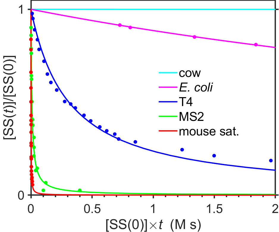
Fig. 7.19 Second-order kinetics of DNA hybridization for DNA sequences from cow (purified non-repetitive DNA fraction), E. coli, T4 bacteriophage, MS2, and mouse satellite. Points show data (from [11]) and lines show best fits to second-order integrated rate law. source
Using the fact that \([\textrm{SS}(t)]=[\textrm{SS}'(t)]\), we can write out the second-order decay, noting that the expression is written as \([\textrm{SS}(t)]/[\textrm{SS}(0)]\) since the researchers generally presented their data as the fraction of remaining single stranded DNA.
As in Section 7.3.3 we can relate rate constant to half-life as follows.
Second-order kinetics predicts that the rate of rehybridization of single-stranded DNA would be sensitive to the concentration of DNA. Since complementary strands of DNA only hybridize with one another, repetitve sequences of DNA would have a much higher effective concentration than a random sequence of DNA. Let’s think a bit about the numbers for this. If a random DNA sequence of approximately the same length as the mouse genome (\(2.5\times10^9\) bp) were chopped into \(10^8\) segments of ~25 bp, then any specific 25 bp DNA sequence would occur with a probability of \(~1/10^{15}\) since \(4^{25}\approx10^{15}\). Thus, fragments of 25 bp or more would be likely to occur only once within a genome of length \(2.5\times10^9\) bp that contains purely random DNA sequences, whereas repetitive DNA sequences would be more abundant. When plotted on a semilogarithmic plot as in Fig. 7.20, it is possible to see just how wide the variation can be for rehybridization kinetics. Note that on a semilogarithmic plot, second-order decays appear as S-shaped curves rather than hyperbolas.
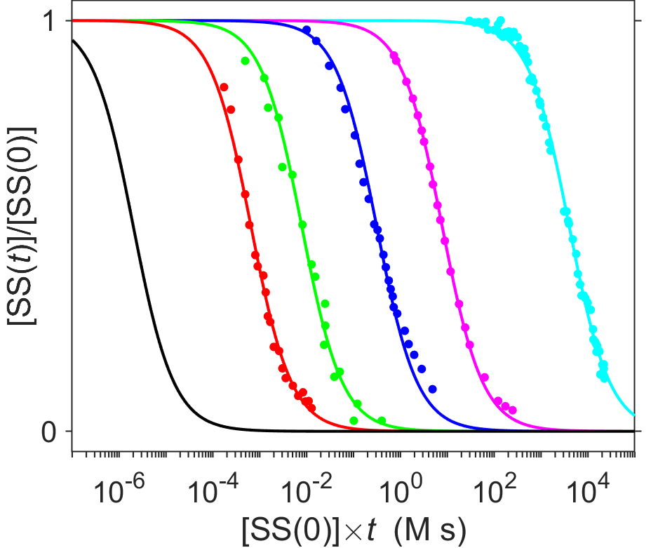
Fig. 7.20 Semilogarithmic plot of DNA hybridization kinetics for data from Fig. 7.19. Points show data (from [11]) and lines show best fit to a second-order integrated rate law. Colors are indicated as cyan=cow (non-repeating fraction), magenta=E. coli, blue=T4 bacteriophage, green=MS2 bacteriophage, red=mouse satellite. The black curve indicates kinetics estimated for the hybridization of poly-A with poly-U.
source
Waring and Britten further used the kinetics of hybridization to estimate the size and copy number of mouse satellite DNA. They found that \([\textrm{SS}(0)]t_{1/2}\) for sheared DNA from the SV40 virus, with a genome length of 6000 bp, was 15 times larger than that of mouse satellite DNA. From this they concluded that at matched concentrations of total single-stranded DNA, the mouse satellite DNA repeat sequence must be ~15 times more abundant than SV40 DNA. This directly implies that the repeat length of the mouse satellite DNA must have a length that is 15 times smaller than the length of the SV40 DNA, that is, the repeat length must be \(6000/15\approx400\) bp. A similar estimate with E. coli DNA yielded an estimate of 320 bp. Finally, using the length of the mouse genome of \(2.5\times10^8\) bp, and the estimate at the time that mouse satellite DNA makes up ~10% of total DNA or 250 million bp (it is now understood to be closer to 5%, for 125 million bp), they concluded that there would be on the order of one million repeats of satellite DNA. Considering the rather indirect methodology, these estimates have held up remarkably well with modern measurements, where the major component of mouse satellite DNA is now believed to contain ~600,000 copies of the 234 bp repeating unit.
Britten and Kohne took this work two steps further [11]. First, they used the highly differing kinetics of reassociation for abundant repetitive sequences, together with the use of hydroxyapatite-based separation of double-stranded DNA from single-stranded DNA, to isolate repetitive sequences from over 50 diverse eukaryotic organisms including humans. Repetitive translocating DNA sequences had been previously reported by Barbara McClintock in corn, and some other repeating DNA sequences were known at the time, but the seeming universality of abundant, repetitive DNA in higher eukaryotes was nonetheless a shock to the scientific community. Second, they introduced the use of the rehybridization assay as a measure of the DNA complexity by calibrating the rehybridization kinetics (Fig. 7.20) to lengths of known sequences of DNA (Fig. 7.21). This was a clever idea since the product \([\textrm{SS}(t)]\) spans about eight orders of magnitude, meaning that the assay has a very large dynamic range.
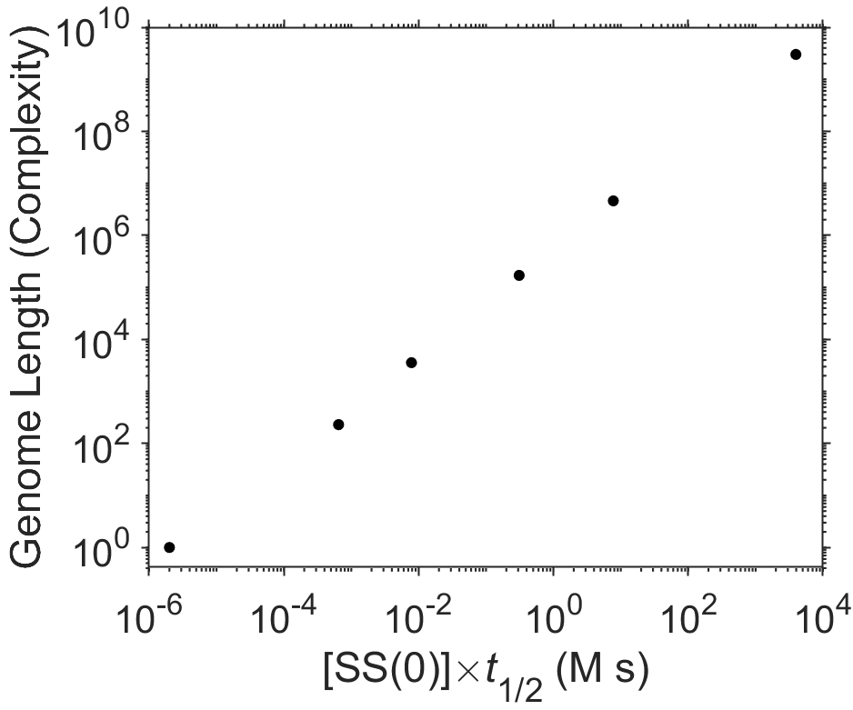
Fig. 7.21 Relationship of genome length or complexity, using modern values, to the product \([\textrm{SS}(t)]t_{1/2}\). Data adapted from [11]. source
Some researchers have even used DNA hybridization kinetics as a method to compare DNA sequences. For instance, Nonoyama and Pagano [12] mixed DNA from Burkitt’s lymphoma patient tumors with DNA from EBV (Epstein-Barr Virus) and were able to see faster hybridization compared to the same experiment using cultured cell DNA and EBV DNA. This was an indirect way without using modern sequencing methods to show that EBV DNA was present in the patient samples, strengthening a case for the association of Burkitt’s lymphoma with infection by EBV. Long before sequencing was a routine affair, DNA hybridization kinetics was a valuable assay for characterizing a genome.
7.8. Problems
7.8.1. Arrhenius + Asparagus
Lau et al. [13] studied the kinetics of the cooking of asparagus and reported that it obeyed Arrehnius kinetics. In one experiment, they measured the rate of textural softening as a function of temperature for tip and base of a spear of asparagus. Use the data in Fig. 7.22, below, to answer the following questions.
At a given temperature, which cooks faster, the bud or the base?
What are the activation energies and pre-exponential factors in the bud and the base?
How long would it take to cook an asparagus bud at 120 °C? (Calculate the half-life of the textural degradation reaction.)
Lau et al. also measured the first-order kinetics of the color changes in asparagus, which becomes a more vivid green upon cooking. Unlike the textural softening that results from the degradation of fiber, the color change results from the conversion of chlorophyll molecules to pheophytin. The authors reported that the color change reaction occurs with an activation energy of \(54\;\textrm{kJ/mol}\) and a rate constant of \(2.2\times10^{-5}/\textrm{s}\) at 98 °C. What is the pre-exponential factor for the color change?
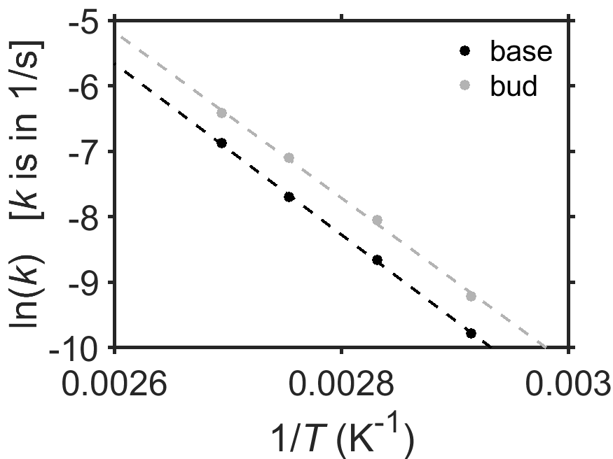
Fig. 7.22 Arrhenius plot of \(\ln(k)\) vs \(1/T\) of the rate of textural softening of asparagus due to cooking. The first-order rate constant \(k\) for rate of textural softening is in units of 1/sec. Data are from [13]. source
ANSWERS
The tip!
Base: \(A=1.2\times10^{12}/\textrm{s}\), \(E_a=105\;\textrm{kJ/mol}\). Base: \(A=2.1\times10^{12}/\textrm{s}\), \(E_a=109\;\textrm{kJ/mol}\).
1 minute
1.4x10^4/s