8. Enzyme Kinetics
What is an enzyme? An enzyme is a catalyst produced by a living organism, usually proteins, but sometimes RNA. Catalase, for example, is an enyzme which catalyzes the reduction of peroxide to water and oxygen. If you have ever used hydrogen peroxide to disinfect a wound and noticed that bubbles form over time, it is because molecules catalase in your blood are acting on the hydrogen peroxide to produce oxygen (and water). Another example is the ribosome, whose catalytic RNA subunit catalyzes peptide bond formation between amino acids. Enzymes work like other catalysts…they accelerate reactions by lowering activation barriers, they are not consumed during a reaction, and they don’t shift the position of the equilibrium. In this chapter we will focus on the kinetics of enzymes.
8.1. Michaelis-Menten Model
The Michaelis-Menten (MM) model of enzyme kinetics a central part of enzymology and biochemistry. Biochemists love to rattle off the \(K_\textrm{M}\), \(k_\textrm{cat}\), \(k_\textrm{cat}/K_\textrm{M}\) values from the Michaelis-Menten model, and understanding these terms is an important part of being ‘enzyme literate’.
8.1.1. Prior Knowledge
Let’s start by reveiwing the observations that led Leonor Michaelis and Maud Menten to develop this model. First, it was known that doubling the amount of enzyme doubled the rate of production of product, so that the rate of product generation was proportional to the amount of enzyme present. Second, larger and larger substrate concentrations typically led to saturation of the inital reaction speed.
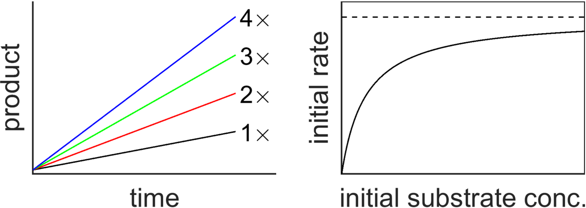
Fig. 8.1 Rate of production of product (slope) is proportional to enzyme concentration (left plot), but saturates for sufficiently large concentrations of substrate (right plot).
The above evidence (Fig. 8.1) rules out a model like \(\require{mhchem}\ce{E+S->E+P}\) since it wouldn’t predict saturation at high substrate concentration, however, the Michaelis-Menten model, which itself was based on a model from Victor Henri, incorporates an intermediate state consisting of a complex between the enzyme and substrate and nicely recapitulates the observed behavior.
In the MM model, an enzyme E and substrate S reversibly bind to form a complex ES, and that complex can irreversibly generate product P while releasing the enzyme for further reaction cycles. This is shown in the chemical scheme, below (note that the scheme is almost the same as was used for diffusion-limited reactions).
Now, before we dive into the math to take a quantitative look at enzyme kinetics, I want to point out that our goals are somewhat different than for most of our work on chemical kinetics where we spent considerable time deriving integrated rate laws. Here, we are less interested in calculating concentrations as a function of time and more interested in studying the rate of enzyme-catalyzed reaction at a given concentration, etc. This is partly since there is not a simple analytical solution to the Michaelis-Menten model and partly since in most biological contexts, enzymes don’t typically consume all of their substrate to exhaustion but operate in conditions somewhat resembling steady-state. So, let’s take a look at steady-state enzyme kinetics with the perspective that we want to see how quickly enzyme-catalyzed reactions can proceed.
8.1.2. Derivation of Basic Michaelis-Menten Kinetics
Here is an outline of the key steps for our derivation. First, we will identify that we want to find enzyme speed \(v\) which we define as the rate of change of product with respect to time, or \(v=\dfrac{d[\textrm{P}]}{dt}\); in turn, this rate of change is proportional to the concentration of the enzyme substrate concentration times the rate constant \(k_\textrm{cat}\) for the catalytic step, or \(v=\dfrac{d[\textrm{P}]}{dt}=k_\textrm{cat}[\textrm{ES}]\). Second, we will make the steady-state approximation that the concentration of the enzyme substrate complex is approximately zero \(\left( \dfrac{d[\textrm{ES}]}{dt}=0 \right)\) in order to solve for the steady-state concentration of the enzyme-substrate complex \([\textrm{ES}]\). From there, we can substitute \([\textrm{ES}]\) and simplify the result.
We can begin with the combined rate law (Eq. (7.2)) for the enzyme-substrate complex \(\textrm{ES}\) which is involved in three parallel reactions. All reactions are modeled as being first-order with respect to all of their respective reactants. Under steady-state conditions, the concentration of \(\textrm{ES}\) is approximately constant, so its rate of change is zero.
We can solve for \([\textrm{ES}]\) under steady state conditions to get
It is customary to combine the three constants together in terms of the Michaelis-Menten constant
in which case our expression for \([\textrm{ES}]\) becomes
In principle, we could use the above expression for \([\textrm{ES}]\) to solve for enzyme speed with \(v=\dfrac{d[\textrm{P}]}{dt}=k_\textrm{cat}[\textrm{ES}]\), but that would put speed in terms of unbound enzyme \(\textrm{E}\) which is inconvenient; we would rather have an expression in terms of total enzyme concentration \(\textrm{E}_0\). We can do so by using a ‘conservation of enzyme’ statement that at any point in time the total concentration of enzyme \([\textrm{E}_0]\) is equal to the sum of the concentrations of unbound enzyme \([\textrm{E}]\) and substrate-enzyme complex \([\textrm{ES}]\)
From there, our expression for \([\textrm{ES}]\) becomes
We can collect the \([\textrm{ES}]\) tems together
and then solve for \([\textrm{ES}]\) to get
This expression for \([\textrm{ES}]\) is now more conveniently in terms of total enzyme concentration \([\textrm{E}_0]\) and can be substituted into our enzyme speed equation to get.
Next, let’s recognize that the maximum speed achievable by the enzyme, \(V_\textrm{max}\), would be achieved if the concentration of the enzyme-substrate complex \([\textrm{ES}]\) were equal to the total enzyme concentration \([\textrm{E}_0]\), or
From this, we can write the customary statement for the Michaelis-Menten model of enzyme kinetics
Let’s take a moment to examine the equation and to think about its meaning. It tells us that the speed \(v\) (rate of generation of product, in the steady-state approximation) is proportional to the maximum achievable speed \(V_\textrm{max}\) (Eq. (8.4)) times a fraction. That fraction can be rewritten as \(\dfrac{1}{K_\textrm{M}/[\textrm{S}]}\) to hopefully clearly indicate that the maximum value of the fraction is 1 and is achieved as the substrate concentration \([\textrm{S}]\) grows very large; this accounts for the saturation behavior. When \([\textrm{S}]=K_\textrm{M}\), the fraction equals 0.5, so that the achieved speed is half of the maximum possible speed.
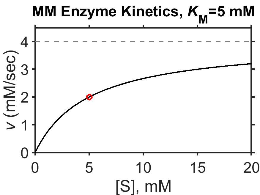
Fig. 8.2 Simulated Michaelis-Menten enzyme kinetics for \(V_\textrm{max} = 4 \textrm{ mM/sec}\) (dashed line), \(K_\textrm{M} = 5 \textrm{ mM}\). The red circle indicates the point where the speed equals half the maximum speed and where, along the x-axis, \([\textrm{S}] = K_\textrm{M}\). source
Sometimes it can be tricky when examining a plot to estimate \(K_\textrm{M}\) by eye, in particular, since the value of \(V_\textrm{max}\) may not be evident. In a research setting, measured \(v\) vs \([\textrm{S}]\) data could be fit with the Eq. (8.5) in order to computationally determine \(K_\textrm{M}\). Historically, and still occasionally today, researchers use techniques to ‘linearize’ the Eq. (8.5) such that the key parameters can be more easily obtained from the slope and y-intercept. The most common of these linearization techniques is the Lineweaver-Burk plot [19] which consists of a plot of \(1/v\) vs \(1/[\textrm{S}]\).
Looking mathematically, one can see how reciprocal speed \(1/v\) yields a line based on the reciprocal Michaelis-Menten equation
In this linearized form, the y-intercept of the plot is equal to \(1/V_\textrm{max}\) and the slope is equal to \(K_\textrm{M}/V_\textrm{max}\) as can be seen in Fig. 8.3, below.
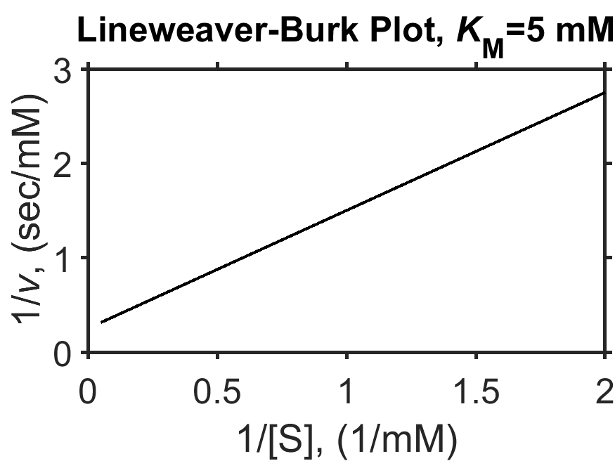
Fig. 8.3 Simulated Michaelis-Menten enzyme kinetics (\(V_\textrm{max} = 4 \textrm{ mM}\), \(K_\textrm{M} = 5 \textrm{ mM}\), as in Fig. 8.2) shown as a Lineweaver-Burk plot of \(1/v\) vs \(1/[\textrm{S}]\). The y-intercept is equal to \(1/V_\textrm{max}\) and the slope is equal to \(K_\textrm{M}/V_\textrm{max}\). source
8.1.3. Competing Substrates
Let’s analyze the case for an enzyme that can act on two substrates. We will see that \(k_\textrm{cat}/K_\textrm{M}\) is a measure of the catalytic efficiency of the enzyme and is sometimes used to describe the specificity of an enzyme (e.g., for one substrate vs another). Note that we can’t use our Eq. (8.5) since for the conservation of enzyme step we assumed in our derivation (Section 8.1.2) that only one substrate can bind the enzyme not two. Instead, we will put the rate here in terms of free enzyme since that is the species for which the two substrates are competing. Starting from our previous MM result for enzyme substrate concentration
Consider the situation where enzyme \(\textrm{E}\) is in the presence of two substrates, \(\textrm{S}_\textrm{A}\) and \(\textrm{S}_\textrm{B}\). We can write a modified MM model for this as
We are interested to compare the speed of conversion for one substrate vs the other. As (above), we will consider the steady state approximation which would hold true for any substrate, symbolized below as \(i\)
which provies the steady-state concentration of enzyme-substrate complex \(\textrm{ES}\) in terms of unbound enzyme \(\textrm{E}\)
Since \(v_i=\dfrac{d[\textrm{P}_i]}{dt}=k_{\textrm{cat},i}[{\textrm{ES}_i}]=\dfrac{ k_{\textrm{cat},i}[\textrm{E}][\textrm{S}_i] }{ K_{\textrm{M},i} }\), we can simply compare the ratio of \(v_\textrm{A}\) to \(v_\textrm{B}\) to see how the competition plays out, noticing that the concentration of unbound enzyme \([\textrm{E}]\) drops out of the ratio.
In this case we can see that for equal concentrations of substrates, it is the ratio \(k_{\textrm{cat},i}{ K_{\textrm{M},i} }\) that dictates specificity, and that the enzyme with the larger value of \(k_{\textrm{cat},i}{ K_{\textrm{M},i} }\) will be favored when the substrate concentrations are matched.
8.1.4. Energy Considerations
Let’s take a brief look at the energy of an enzyme-catalyzed reaction along a somewhat notional ‘reaction coordinate’. The cartoon, below (Fig. 8.4), shows that the uncatalyzed reaction and the catalyzed reaction have the same respective energies for the reactants and products; as a result, enzymes, like other catalysts, do not shift the position of equilibrium (Section 7.5). We can also see from the cartoon that the catalyzed reaction has a lower activation energy that can lead to very substantial increase in speed of the reaction. Finally, we can also see that the enzyme-substrate complex, ES, is separated from reactants and products by activation barriers.
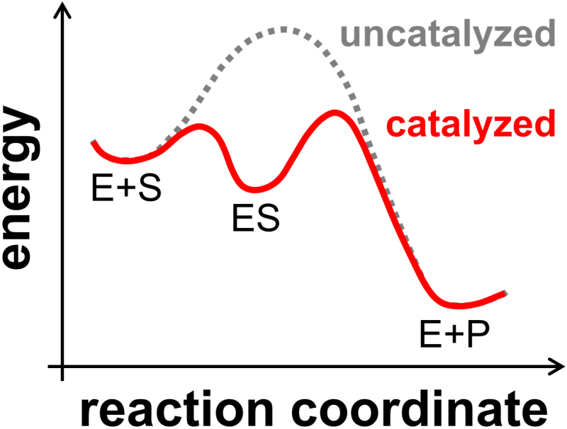
Fig. 8.4 Cartoon of energy along reaction coordinate for a reaction with and without the presence of an enzyme.
8.1.5. Michaelis-Menten Model and Mechanisms
The MM model, \(v=V_\textrm{max}[\textrm{S}]/(K_\textrm{M}+[\textrm{S}])\), works surprisingly well in exact or slightly modified form for a large number of systems. Note, however, that the MM model is a minimal model and it may omit or simplify many details, including a potentially complex set of intermediates.
In general, the minimal Michaelis-Menten reaction scheme
could be written much more mechanistically in terms of elementary steps with various binding, intermediates, and release steps such as
however, in practice, it is very hard to measure many of these specific intermediates. As a result, the identity of the rate-limiting steps that governs behavior in the Michaelis-Menten model can be challenging to identify. For instance, sometimes the catalytic step is rate-limiting while other times product release is rate-limiting. It is therefore not straightforward to attribute an observed \(k_\textrm{cat}\) from the MM model to the actual catalytic step (e.g., making or breaking a covalent bond) without careful measurements; the same can be said for \(k_1\) and \(k_2\). In addition, when working with more mechanistic models, researchers typically utilize minimal models that are consistent with their level of data while recognizing that additional substeps are likely occurring but that these are not easily detected.
8.2. Enzyme Inhibitors
A huge fraction of drugs are enzyme inhibitors, ranging from everyday medicines, blockbuster drugs, and even some herbicides. Let’s take a brief look at some of these moelcules and note the many ways in which they affect our lives.
Aspirin is an irreversible inhibitor of the enzyme cycloogygenase, and administration of the drug suppresses production of prostaglandin molecules involved in inflammation signaling. Humans consume a whopping >75,000,000 pounds of the painkiller each year.
Penicillin is an irreversible inhibitor of a transpeptidase enzyme that catalyzes crosslinking of the peptidoglycan strands of bacterial cell walls. The antibiotic is estimated to have saved more than 200,000,000 lives since its discovery in the 1920s.
Lipitor is a statin drug that is a competitive inhibitor of the enzyme HMG-reductase that is involved in cholesterol production. The drug significantly lower cholesterol levels and reduce the death rate for people with cardiovascular disease. While Lipitor was under patent protection, it generated > $130,000,000,000 in sales for Pfizer.
Sildenafil, also known as Viagra, is a competitive inhibitor of the enzyme phosphodiesterase and can increase blood flow to the penis as a means of treating erectile dysfunciton. Apparently, sildenafil has also been reported as effective in reducing the duration of jet lag in hamsters [20].
Glyphosate is an herbicide, also known as Roundup, is an uncompetitive inhibitor of the enzyme EPSPS that is involved in biosynthesis of the aromatic amino acids tryptophan, phenylalanine, and tyrosine. Mutant EPSPS that is resistant to glyphosate can be introduced genetically into crops so that broad use of glyphosate can kill unwanted vegetation. In 2011, over 1,000,000,000 pounds of glyphosate was used worldwide. While glyphosate use is somewhat controversial, due in part to the rise of herbicide-resistant “super-weeds” that have been fostered by its heavy use, and due in part to concerns that glyphosate may cause some types of cancer, the herbicide is still widely used.
In this section, we will introduce different classes of reversible enzyme inhibitors, and we will calculate modified Michaelis-Menten kinetics expressions for each. Note that irreversible enzyme inhibitors, such as aspirin, typically operate by covalent modification of an enzyme at or near the active site of the enzyme, resulting in a reduction of the amount of enzyme available. As such, no special derivation is required. Reversible inhibitors are molecules that non-covalently bind an enzyme and come in a few different forms that are kinetically distinguishable as we shall soon see.
8.2.1. Competitive Inhibition
Competitive inhibition. A competitive inhibitor is a molecule that reversibly binds an enzyme, and, while bound, blocks binding of a substrate to an enzyme. Often, competitive inhibitors are molecules that resemble a substrate and bind an enzyme’s active site, but cannot be converted to product. Their net effect is to reduce the speed of product formation by depleting the concentration of enzyme available for catalysis. The reaction scheme for competitive inhibition is shown, below.
At steady state, both \([\textrm{ES}]\) and \([\textrm{EI}]\) are unchanging. As before for the basic MM derivation in steady state we found that
In addition, the steady state condition \(\dfrac{ d[\textrm{EI}] }{ dt } = 0\) leads to
so that
where the dissociation constant is defined as \(K_\textrm{I} = \dfrac{ k_4 }{ k_3 }\). At this point, we deviate from the basic MM derivation by incorporating the enzyme-inhibitor concentration into our conservation of enzyme statement, which is now
We can put the conservation of enzyme statement in terms unbound enzyme concentration \([\textrm{E}]\), substrate concentration \([\textrm{S}]\), and inhibitor concentration \([\textrm{I}]\)
solve for unbound enzyme concentration \([\textrm{E}]\)
and then subsitute into our expression for enzyme-substrate concentration \([\textrm{ES}]\) from above to get
As with the basic MM derivation, using \([\textrm{ES}]\) in terms of \([\textrm{E}_0]\), \([\textrm{S}]\), and \([\textrm{I}]\) we can solve for the reaction speed
As with the basic (uninhibited) MM derivation, we can use the relation \(V_\textrm{max} = k_\textrm{cat}[\textrm{E}_0]\) to get our final expression for enzyme speed in the presence of a competitive inhibitor
Let’s take a minute to examine our result. First, in the case when no inhibitor is present (\([\textrm{I}]=0\)) or the inhibitor binding is very weak (i.e., \(K_\textrm{I}\) is very large), the term \([\textrm{I}]/K_\textrm{I}\) drops out and we obtain the basic (uninhibited) MM equation (Eq. (8.5)). Second, as the substrate concentration grows to be very large, the enzyme speed will approach \(V_\textrm{max}\) as with the basic MM equation. Third, the characteristic half-maximum speed is now obtained when \([\textrm{S}] = K_\textrm{M}\left( 1 + \dfrac{[\textrm{}I]}{K_\textrm{I}} \right)\); in short, the equation has the same shape but is stretched toward larger values of substrate concentration with a magnitute that depends on the inhibitor concentration. For instnace, when \([\textrm{I}]=K_\textrm{I}\), the half-maximum speed occurs for a substrate concentration of \([\textrm{S}]=2K_\textrm{M}\) (try calculating that yourself!).
We can see some of the above points illustrated by examining a plot of enzyme speed in the presence and absence of a competitive inhibitor (Fig. 8.5).
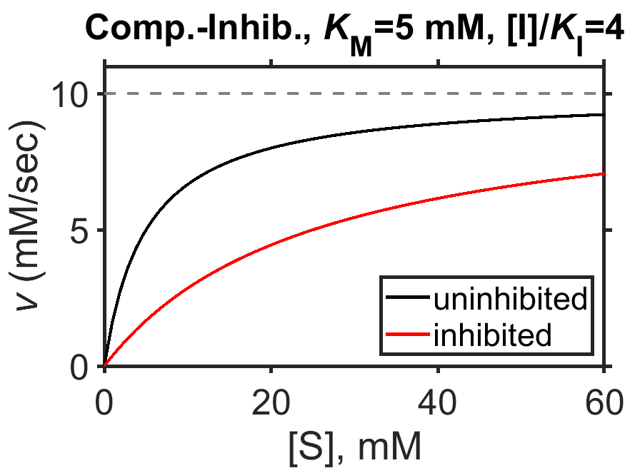
Fig. 8.5 Simulated Michaelis-Menten enzyme kinetics for \(V_\textrm{max} = 10 \textrm{ mM/sec}\) (dashed line), \(K_\textrm{M} = 5 \textrm{ mM}\), in the presence of competitive inhibitor (\([\textrm{I}]/K_\textrm{I}=4\), red curve) and in the absence of competitive inhibitor (black curve).
source
Let’s check what the Lineweaver-Burk form of the MM equation for competitive inhibition will look like. In that case, we have
From the above equation, we can see that the Lineweaver-Burk (\(1/v\) vs \(1/[\textrm{S}]\)) form of the competitive inhibition MM equation again fits the shape of a line but with a larger slope, as is also shown in Fig. 8.6.
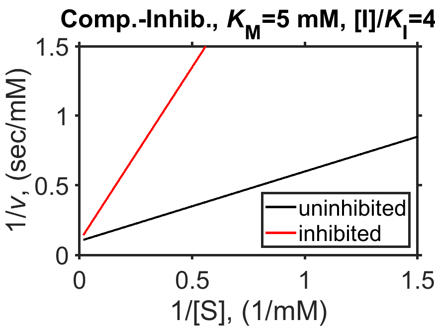
Fig. 8.6 Simulated Michaelis-Menten enzyme kinetics for \(V_\textrm{max} = 10 \textrm{ mM}\) (dashed line), \(K_\textrm{M} = 5 \textrm{ mM}\), in the presence of competitive inhibitor (\([\textrm{I}]/K_\textrm{I}=4\), red line) and in the absence of competitive inhibitor (black line); shown as a Lineweaver-Burk plot of \(1/v\) vs \(1/[\textrm{S}]\).
source
8.2.2. Uncompetitive Inhibition
Uncompetitive inhibition. An uncompetitive inhibitor is a molecule that reversibly binds an enzyme and, while bound, prevents the conversion of substrate to product. One way this might occur is for enzymes that require two substrates, with the inhibitor binding to one of th esites, but examples are known for single-substrate enzymes are known in the literature (e.g., the inhibition of alkaline phosphatase by phenylalanine). As we will see, uncompetitive inhibition is kinetically distinct from competitive inhibition.
The reaction scheme for uncompetitive inhibition is shown, below.
Our derivation will follow almost the same path as for competitive inhibition, above, starting wiht the steady state approximation that for \([\textrm{ES}]\)
In addition, the steady state condition \(\dfrac{ d[\textrm{ESI}] }{ dt } = 0\) leads to
so that
where the dissociation constant for uncompetitive inhibition is defined as \(K_\textrm{I'} = \dfrac{ k_6 }{ k_5 }\). Again, as before, we will use a conservation of enzyme statement to put the rates in terms of total enzyme \(\textrm{E}_0\) rather than unbound enzyme \(\textrm{E}\).
Substituting in expressions for \([\textrm{ES}]\) and \([\textrm{ESI}]\) gives us
which we can simplify as
and rearrange to get \([\textrm{E}]\) in terms of \([\textrm{E}_0]\)
With our expression, above, for \([\textrm{E}]\), we can now solve for the reaction speed
As before, we can use the relation \(V_\textrm{max}=k_\textrm{cat}[\textrm{E}_0]\) to get our final expression now for enzyme speed in the presence of an uncompetitive inhibitor.
In the presence of an uncompetitive inhibitor, let’s take a look to see that the effective maximum speed is decreased regardless of substrate concentration, while the concentration of substrate \([\textrm{S}]\) at which the reaction reaches half of its effective maximum speed is decreased from \(K_\textrm{M}\). We can perhaps see both of these trends mathematically by dividing top and bottom by the term \(\left( 1 + \dfrac{ [\textrm{I}] }{ K_\textrm{I'} } \right)\), which gives us
In the above expression, hopefully it is clear that as \([\textrm{S}]\) grows very large, the maximum achievable speed is reduced from \(V_\textrm{max}\) in the presence of an inhibitor to be \(\dfrac{ V_\textrm{max} }{ 1+\dfrac{[\textrm{I}]}{K_\textrm{I'}} }\). In a similar way, the concentration of substrate \([\textrm{S}]\) at which half the maximum achievable speed is attained occurs when \([\textrm{S}] = \dfrac{ K_\textrm{M} }{ 1+\dfrac{[\textrm{I}]}{K_\textrm{I'}} }\).
The above points are evident from examining a plot of enzyme speed in the presence and absence of an uncompetitive inhibitor (Fig. 8.7). There, we can see that for high substrate concentration, the plateau is lower than \(V_\textrm{max}\) and that half of the effective maximum speed is achieved for a concentration of substrate of ~2.5 mM.
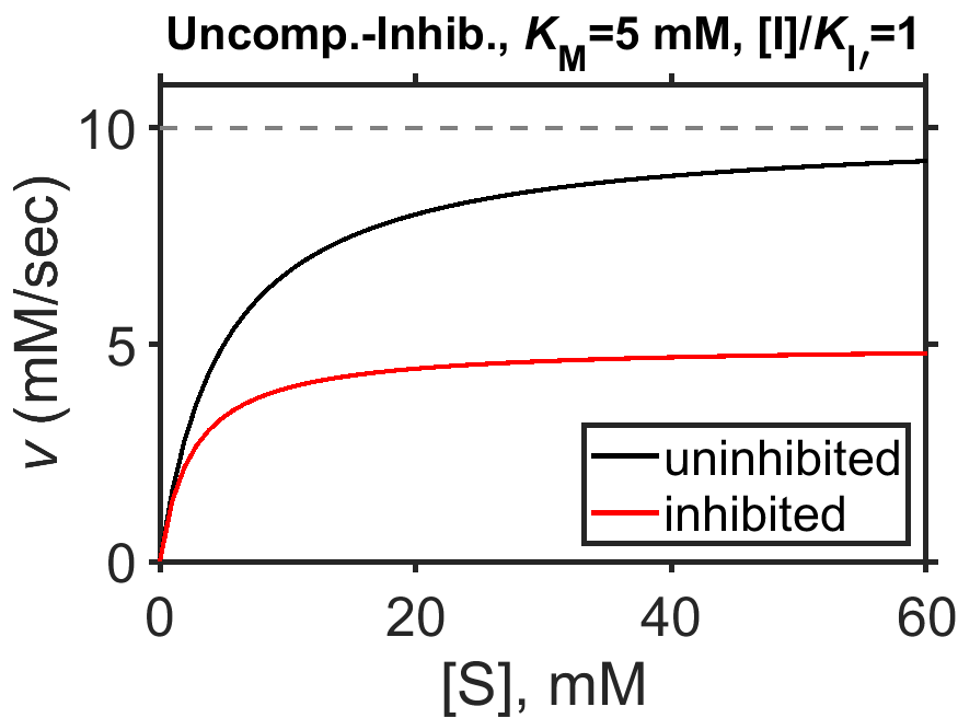
Fig. 8.7 Simulated Michaelis-Menten enzyme kinetics for \(V_\textrm{max} = 10 \textrm{ mM/sec}\) (dashed line), \(K_\textrm{M} = 5 \textrm{ mM}\), in the presence of uncompetitive inhibitor (\([\textrm{I}]/K_\textrm{I}=1\), red curve) and in the absence of uncompetitive inhibitor (black curve).
source
The Lineweaver-Burk form of the MM equation for uncompetitive inhibition is shown below, having the same slope regardless of amount of inhibitor present but a larger y-intercept in the presence of inhibitor as shown in Fig. 8.8.
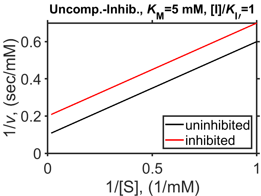
Fig. 8.8 Simulated Michaelis-Menten enzyme kinetics for \(V_\textrm{max} = 10 \textrm{ mM/sec}\) (dashed line), \(K_\textrm{M} = 5 \textrm{ mM}\), in the presence of uncompetitive inhibitor (\([\textrm{I}]/K_\textrm{I}=1\), red curve) and in the absence of uncompetitive inhibitor (black curve); shown as a Lineweaver-Burk plot of \(1/v\) vs \(1/[\textrm{S}]\).
source
8.2.3. Mixed Inhibition
In principle, one reversible inhibitor could have multiple effects. One way for this to occur is for the inhibitor to bind to a site other than the active site, but also inhibit binding of the substrate through changes to the enzyme’s structure. The result is a combination of reversible competitive inhibition and reversible uncompetitive inhibition. (Sometimes people call this non-competitive inhibition; other times only the special case of \(K_\textrm{I}=K_\textrm{I’}\) is called non-competitive. I prefer avoiding the term since non-competitive actually still has inhibitor competing for active site and the term sounds a lot like uncompetitive which can be confusing.)
The mixed inhibition reaction scheme is just the combination of the competitive inhibition and uncompetitive inhibition reaction schemes, shown below.
The result, using the same basic procedures as above for competitive and uncompetitive inhibition derivations, above, is shown below. Try calculating it yourself!
8.2.4. Summary
Here is a summary of our key results on Michaelis-Menten kinetics.
Summary of Michaelis-Menten Kinetics Results
\(k_\textrm{cat}\) is the first order rate constant for \(\ce{ES ->[k_\textrm{cat}] E + P}\) with units of 1/sec.
\(K_\textrm{M}\) is the MM constant in units of concentration. In the absence of inhibitor, it equals the concentration of substrate that gives half the maximum speed \(V_\textrm{max}\).
\(V_\textrm{max} = k_\textrm{cat}E_0\) where \(V_\textrm{max}\) is the maximum achievable speed in the case that all enzyme is bound by substrate, in units of \(\textrm{M}/\textrm{sec}\).
The uninhibited MM-kinetics are described by \(v_\textrm{no inhibitor} = \dfrac{ V_\textrm{max} [\textrm{S}] }{ K_\textrm{M} + [\textrm{S}] }\)
Inhibitors give distinct kinetic signaturs depending on the mechanism(s) of inhibition.
An irreversible inhibitor binds, typically covalently, to an enzyme to convert it to an inactive form.
A competitive inihbitor reversibly blocks binding of substrate to enzyme via \([\textrm{EI}] = \dfrac{ [\textrm{E}][\textrm{I}] }{ K_\textrm{I}}\). The MM kinetics are described by \(v_\textrm{competitive inhibitor} = \dfrac{ V_\textrm{max}[\textrm{S}] }{ K_\textrm{M} \left( 1 + \dfrac{[\textrm{I}]}{K_\textrm{I}} \right) + [\textrm{S}] }\)
An uncompetitive inihbitor reversibly blocks conversion of substrate to product via \([\textrm{ESI}] = \dfrac{ [\textrm{ES}][\textrm{I}] }{ K_\textrm{I'}}\). The MM kinetics are described by \(v_\textrm{uncompetitive inhibitor} = \dfrac{ \dfrac{V_\textrm{max} }{ 1 + \dfrac{ [\textrm{I}] }{ K_\textrm{I'} } } [\textrm{S}]}{ \dfrac{ K_\textrm{M} }{ 1 + \dfrac{ [\textrm{I}] }{ K_\textrm{I'} } } + [\textrm{S}] }\)
A mixed inhibitor can operate simultaneously as a competitive or an uncompetitive inhibitor. The MM kinetics are described by \(v_\textrm{mixed inhibition} = \dfrac{ V_\textrm{max}[\textrm{S}] }{ K_\textrm{M} \left( 1 + \dfrac{[\textrm{I}]}{K_\textrm{I}} \right) + [\textrm{S}] \left( 1 + \dfrac{ [\textrm{I}] }{ K_\textrm{I'} } \right) }\)
Lineweaver-Burk plots are useful for studying enzymes & enzyme inhibitors, and are commonly encountered in the literature, but are not good to use for curve-fitting purposes in a research context.