3. Entropy and the Second Law
3.1. Time’s Arrow
Let’s start with a question. Can a ball roll up a hill? Most of the time when I ask this to students, they say no. However, if I then ask students whether they could kick a ball uphill, they recognize that they can and that a ball can indeed roll uphill. A careful look at Newton’s equations of motion reveals that they work just as well forward and backwards. Despite this, we have a very good intuition of how things should progress in time: gases expand in a vacuum; heat is transferred from hot objects to cold ones; breaking of glass creates many tiny pieces that don’t put themselves back together, etc. Extending these ideas to chemical processes, we know that salt will dissolve in water, not the reverse, and that iron in the presence of oxygen will rust, not the reverse, etc. So what is it that governs the direction of events? What is the guiding principle governing the direction of these processes? Is it just energy? No! The second law of thermodynamics—one of the most important laws in all of science—tells us which direction of an event will occur. This concept is called time’s arrow.
3.2. Second Law
The Second Law is concerned with entropy and states the following.
Entropy, \(S\) is a state function and can be calculated using \(dS=\dfrac{dq_\textrm{rev}}{T}\). The subscript ‘rev’ indicates that a reversible path must be used for the calculation.
The change in entropy in any process is given by \(dS \ge \dfrac{dq}{T}\), where \(>\) is used for a sponaneous (irreversible) process and \(=\) is used for a reversible process.
There are many alternative statements of the second law. We will visit this further in section Section 3.9, below, but for now let us also consider the following.
The entropy of an isolated system increases for irreversible (spontaneous) processes and is zero for a reversible process.
Since the universe is like a really big isolated system, we can say that any spontaneous event that occurs increases the entropy of the universe. We will take some time to unpack the second law and entropy over the next few sections.
3.3. Entropy and State Functions
We saw in Section 2 that both work and heat are path functions. Let’s use the first law to consider whether the quantity \(dq/T\) is a state function for an ideal gas. Note that the second law says entropy is a state function for all substances, but the ideal gas is perhaps the easiest to use for a test calculation.
We can start with the differential form of the first law and then substitute the differential of work \(dw = -PdV\) and the ideal gas law \(V=nRT/P\).
so that
Next, let’s use Euler’s test for exactness to confirm that \(dq\) is a path function, as expected. To test \(q\) for exactness we want to see whether the order of derivatives matters for \(q\) with respect to \(T\) and \(V\).
This process will be easier if we recognize from Eq. (3.1), above, that \(\left( \frac{\partial q}{\partial V} \right)_T = \frac{nRT}{V}\) and that \(\left( \frac{\partial q}{\partial T} \right)_V = n\overline{C}_V\). If we differentiate each term with respect to the other variable, \(V\), or \(T\), then we obtain
and
Since taking the derivative of \(q\) first with respect to \(T\) and then \(V\) gave a different result than for the other order (\(V\) and then \(T\)), we can conclude that \(q\) is a path function as expected. Now, let’s take a look at this for entropy as defined mathematically in the second law as \(dS=dq/T\). In the equation, below, we will use our differential of \(q\) from Eq. (3.1), above.
This time, from Eq. (3.2), we can see that \(\left( \frac{\partial S}{\partial V} \right)_T = \frac{nR}{V}\) and that \(\left( \frac{\partial S}{\partial T} \right)_V = \frac{n\overline{C}_V}{T}\). If we differentiate each term with respect to the other variable, \(V\) or \(T\), we now obtain
and
so we can see that entropy is indeed a state function as expected since the partial derivatives of \(S\) with respect to \(V\) then \(T\) or \(T\) then \(V\) give the same answer. While this example was derived specifically for an ideal gas, the second law tells us that this is true for all substances.
3.4. What Is Entropy?
Many students learn in prior courses that entropy is a measure of disorder. I suppose this is on the right track, and that if you were limited to defining entropy with only one other word, then disorder would probably be the best choice. However, it is too limiting to equate entropy with disorder, and we will take a closer look to better understand the subtleties of entropy.
Rigorously defined, entropy is a measure of the number of (quantum mechanically) available configurations of a system. From this perspective we can see that the second law says that a system tends to move toward the most probable state and that this guides our understanding of time’s arrow. A perhaps unfamiliar aspect of entropy is that unlike energy, entropy is not conserved in the sense that the entropy of the universe is always increasing.
3.4.1. Statistical View of Entropy
Let’s look at an example to illustrate number of available configurations using a box containing four particles and where the particles can be on either side of a partition within the box (Fig. 3.1). We will refer to a macrostate here as the number of balls on each side of the partition, where there are five possible macrostates (all balls on left, three balls on left, two on left, one on left, and all balls on right). For each macrostate, we can then look to see how many microstates there are that can achieve the macrostate. There is only one way to arrange all four particles on one side or the other, but there are four ways to arrange one particle on either side, and there are six ways to arrange a 50/50 split. With this perspective, the macrostate with a 50/50 split has six possible microstates would have higher entropy and would also be more probable than any other macrostate. In contrast, all microstates are equally probable.
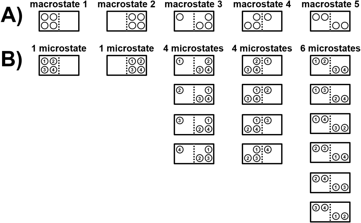
Fig. 3.1 A box contains four particles that can exist on either side of a partition. A) There are five possible macrostates for a system that describe how many balls are on each side of the partition. B) Each macrostate can be achieved by 1-6 microstates. A macrostate with more possible microstates has a higher entropy.
When we generalize this result to a large number of particles, we see that the probability of finding all the particles on one side of the box is vanishingly small. Even finding 50.001% of the particles on one side is extremely unlikely for a mole of particles. Let’s try a couple examples of this sort of calculation.
Example 1. What is the chance that 10 ideal gas particles are all in the left half of a box?
Ideal gas particles are independent and infinitesimal and assumed to be randomly distributed on either side of the box. Each particle will have a probability of 1/2 of being in the left half of the box. So for one particle the chance is \(\frac{1}{2}\). For two particles it is \(\left( \frac{1}{2} \right)^2=\frac{1}{4}\) and for 10 particles it is \(\left( \frac{1}{2}\right)^{10}=\frac{1}{1024}\). So the chance is ~0.1% that all 10 gas particles spontaneously ‘order’ themselves on one side of the box. While waiting long enough to observe such a phenomenon may seemingly violate the second law of thermodynamics, it is really a consequence of not studying a ‘sufficiently large’ ensemble of particles, and in fact a ~1/1000 chance is not so small.
Example 2. What is the chance that one mole of ideal gas particles are all in the left half of a box?
The probability of this will be \(\left( \frac{1}{2} \right)^{6.02\times10^{23}}\), which is a really really really small number. It is approximately \(10^{-100,000,000,000,000,000,000,000}\). That’s right, \(1\) divided by \(10\) raised to the power of 100,000,000,000,000,000,000,000. It is an unimaginably small number…so small that it tells you the scenario will not occur.
Example 3. What is the chance that one mole of ideal gas particles compress themselves by just a tiny, tiny bit, say by just 0.0001%? That is, what is the probability that the gas particles could spontaneously occupy a volume just one millionth part smaller than the box itself? That seems like a much less dramatic ‘ordering’ of the system than sticking the particles all on one half of the box. For one particle the chance of existing in the left 999,999/1,000,000 fraction of the box is \(0.999999\). For two particles the chance is \(0.999999^2\). For a mole of particles the chance will be \(0.999999^{6.02*10^{23}}\) which is still a really, really small number, or \(\sim 1\) in \(10^{100,000,000,000,000,000}\). If we wanted to wait for this scenario to occur, how long would it take? Well if we could adopt a new configuration every \(10^{-13}\) seconds (very roughly the time it takes one gas particle to travel the diameter of a hydrogen atom) then even in the entire age of the universe (\(\sim 10^{17}\) seconds) we would only have a reasonable chance to observe things that have a probability of \(1\) in \(10^{30}\) or higher. Our probability was \(\sim 1\) in \(10^{100,000,000,000,000,000}\) which is waaaaaayyyyy smaller. Basically, it ain’t gonna happen.
3.4.2. Boltzmann’s Entropy Equation
Ludvig Boltzmann was a physicist who did groundbreaking work on thermodynamics and statistical mechanics in the late 1800s and early 1900s. He died tragically of suicide amid protracted controversey surrounding his ideas, which became widely accepted not long after his death. He was buried in Vienna, and at the very top of his gravestone is inscribed a famous equation known as the Boltzmann entropy equation that relates entropy to number of available microstates.
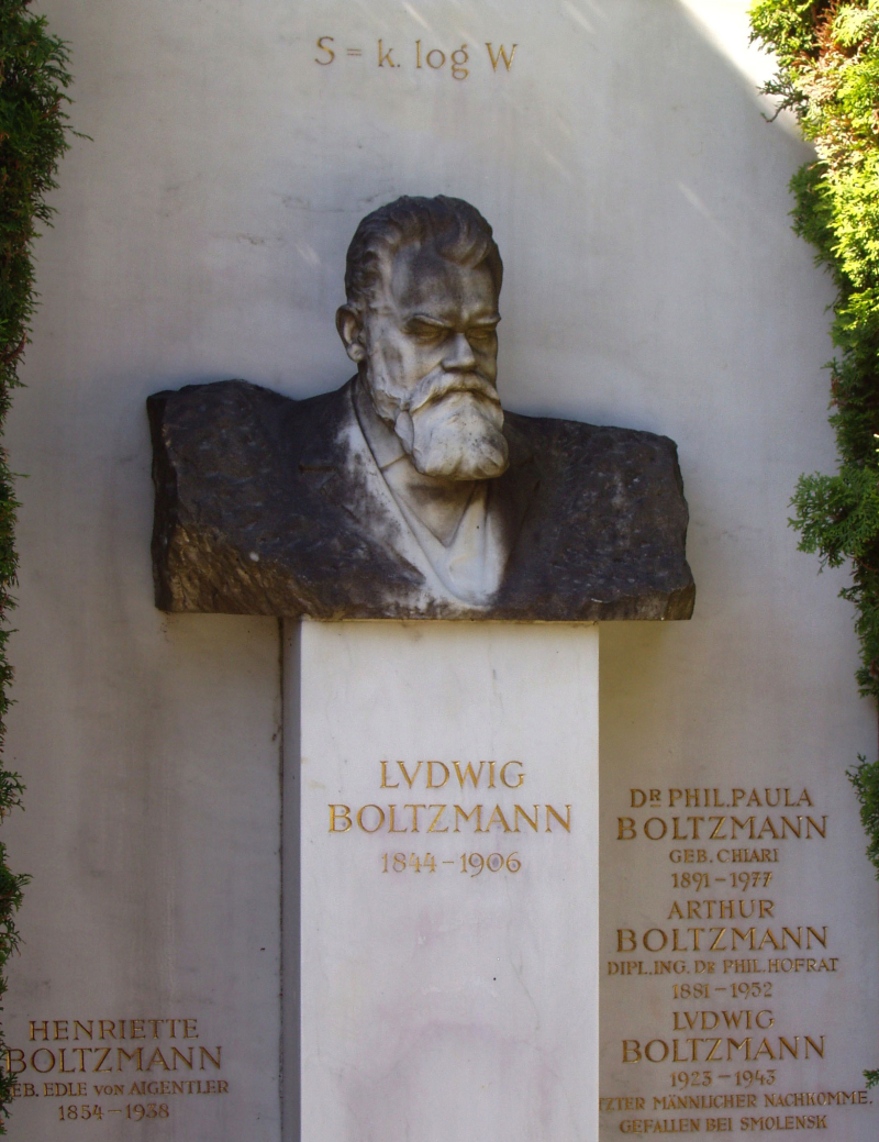
Fig. 3.2 Grave of Ludvig Boltzmann in Vienna, Austria, bearing his entropy equation. (Photo from Daderot, under a CC-BY 3.0 license via Wikipedia.)
Boltzmann’s entropy equation (Eq. (3.3)) states
It says that entropy is an absolute quantity whose value is the product of the natural logarithm of the number of (quantum mechanical) states available to the system, \(W\), multiplied by \(k_\textrm{B}\), where \(k_\textrm{B}\) is Boltzmann’s constant, or just the gas constant divided by Avogadro’s number in uints of \(\textrm{J/K}\). Boltzmann’s entropy equation shows us quantitatively that there is a logarithmic dependence of entropy on the number of available microstates and it reveals that the units of entropy are \(\textrm{J/K}\).
3.4.3. Disorder vs Entropy
Let’s return to the suitability of the term ‘disorder’ using an example contrast disorder, which is notional and nonquantitative, and number of available configurations. The cartoons in Fig. 3.3 illustrates one way in which increasing entropy can actually produce order of sorts. The yellow balls have an excluded volume (gray) that cannot be occupied by the (centers of) the much more numerous smaller black balls. That excluded volume can be minimized if the yellow balls aggregate and/or stick to the walls of the container, as shown on the right, and the reduction in excluded volume can be entropically driven without any attractive or repulsive inter-particle forces beyond the hard boundaries of the balls. This means that while the yellow balls appear more disordered on the left, the overall entropy is actually higher on the right side with the ordered yellow balls. This is because in the right the black balls have more volume available.
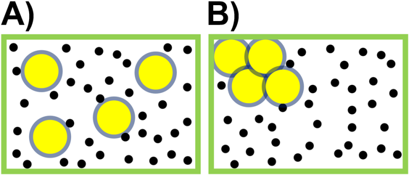
Fig. 3.3 A box contains a few large yellow balls and more numerous small black balls. So-called depletion forces tend to cause the randomly distributed large yellow balls in A) to aggregate as in B) in order to reduce the excluded volume with minimal loss of translational entropy.
From this example, I hope you can see that the notion of entropy as ‘disorder’ is not very good. The (natural log of the) number of available configurations is a more accurate and quantitative way to think about entropy, so in that context, the second law says that an isolated system will go towards a state where it has the maximum number of available configurations. We will talk more below about absolute entropy and how to calculate entropy changes, which may help you gain a better feeling for entropy. Many students struggle with the concept of entropy, and it is covered in greater microscopic deail in courses such as statistical mechanics.
3.5. Key Entropy Calculations
Entropy is a state function and in some circumstances, one can find tabulated values for the entropy of various substances and can calculate entropy changes analogous to enthalpy changes. Entropy changes can also be calculated using the second law’s mathematical statement \(dS=dq_\textrm{rev}/T\). If calculating analytically, you need to be sure to use a reversible path to connect the initial and final states of the system. If the actual path for the process is irreversible, your job will be to find an alternate reversible path between those initial and final states of the system. In many problems, you will not be provided with information indicating that a specific process is reversible or irreversible (see Section 2.8). Instead, you will need to consider the situation and use the available information to determine whether a process is reversible. In the case of an irreversible process, you will need to identify an alternative reversible path connecting the same initial and final states for the process under consideration.
Example 1. One mole of solid water melts at 273 K, 1 atm. What are \(\Delta S_\textrm{sys}\), \(\Delta S_\textrm{surr}\) and \(\Delta S_\textrm{univ}\)? The heat of fusion of water is \(\Delta H^\circ_\textrm{fus}=6.01 \textrm{ kJ/mol}\).
We know that at 1 atm, the equilibrium melting temperature of water is 273 K, so we can conclude that this process is reversible and we can calculate along the real path. Our basic strategy is to integrate the mathematical statement of the second law \(dS=dq_\textrm{rev}/T\). As with enthalpy calculations, we need to be careful to manually insert the sign of the enthalpy of transformation, such as the enthalpy of fusion in this case which will have a positive sign as tabulated for a melting process (but it would have a negative sign for freezing, see Section 2.3.2).
The entropy change of the system is positive because liquid water has a higher number of configurations than solid water at the same temperature. Now, what about the entropy change of the surroundings and universe? We can calculate \(\Delta S_\textrm{surr}\) by using \(q_\textrm{surr}=-q_{sys}\). This process is assumed to occur at a constant temperature, as if the surroundings were a very large thermal bath at 273 K. In this case, we expect the entropy change of the surroundings to simply be given by \(\Delta S_\textrm{surr}=-\Delta S_\textrm{sys}\).
From this we can easily conclude that the entropy change of the universe would be zero since \(\Delta S_\textrm{univ}=\Delta S_\textrm{sys}+\Delta S_\textrm{surr}\). Here is a kind of spoiler… all reversibe processes have zero entropy change for the universe. It is important on a fundamental level to recognize that reversible processes have \(\Delta S_{\textrm{univ}}=0\), and it is also helpful on a practical level since it can save time in calculations.
Practice entropy change calculation for a phase change.
Question: Two moles of water vapor condense to liquid water at 373 K, 1 atm. What are \(\Delta S_\textrm{sys}\), \(\Delta S_\textrm{surr}\) and \(\Delta S_\textrm{univ}\)? The heat of vaporization of water is \(\Delta H^\circ_\textrm{vap}=40.7 \textrm{ kJ/mol}\).
Answer: First, notice that this process is happening reversibly since the equilibrium boiling/condensation temperature of water at 1 atm is 373 K. This means we do not need to calculate along an alternative reversible path. Second, we will be careful, below, to manually insert a negative sign into the numeric value of the enthalpy of vaporization since condensation will have a negative value but enthalpies of phase transformations are just tabulated positive (see Section 2.3.2).
The entropy change of the system, here, is negative, reflecting the fact that liquid water at 373 K has a lower entropy than gaseous water at the same temperature. While liquid water molecules are able to diffuse relative to one another, the liquid molecules are still bound to one another in contrast to water molecules in a gas which are not bound. This explains the negative entropy sign for water when condensing from a gas to a liquid. Additionally, this is a reversible process so we know that \(\Delta S_\textrm{uinv}=0\) and \(\Delta S_\textrm{surr}=-\Delta S_\textrm{sys}=218 \textrm{ J/K}\).
Example 2. Calculate the change in entropy of the system due to the gradual cooling of 1 mol of solid water from 273 K, 1 atm to 263 K, 1 atm. The heat capacity of ice is 38 J/(K mol) and we assume it to be temperature-independent here.
The problem statement indicates that the process is gradual which is a hint that the process is reversible and no alternative path is required. We can calculate the entropy change for the system by integrating the mathematical statement of the second law \(dS=dq_\textrm{rev}/T\).
Example 3. Calculate the entropy change of the system when 1 mol of ideal gas is heated slowly from 300 K to 600 K at constant volume. What is the entropy change of the surroundings? The universe?
This process is indicated as happening slowly, which we will interpret to mean that the process is happening reversibly and at equilibrium and that we do not need to calculate along an alternative reversible path.
Intreasing the temperature of an object increases its entropy, so the entropy change of the system here was positive. Also, for any reversible process, we know that \(\Delta S_\textrm{uinv}=0\) and that \(\Delta S_\textrm{surr}=-\Delta S_\textrm{sys}=-8.64 \textrm{ J/K}\).
Example 4. Calculate the entropy change when 1 mol of ideal gas is compressed reversibly at a constant temperature of 400 K from 20 L to 10 L.
As before, we will integrate the mathematical statement of the second law \(dS = dQ/T\). In order to determine \(dq\) we will notice that if the temperature is constant, then \(dU=0\), and that \(dq=-dw\). We can use the differential form of work (see Section 2.9) as \(dw=-PdV\) to give \(dq=PdV\) and then use this when we integrate the second law together with the ideal gas law as shown below.
The negative entropy change of the system here reflects the fact that the volume of the container decreased while the system was maintained at a constant temperature, so there were fewer possible configurations within a smaller volume.
Practice entropy change calculation for reversible constant pressure heating of an ideal gas.
Question: 3 moles of ideal gas are gradually heated from 250 K to 400 K at a constant pressure of 125,000 Pa. What is the change in entropy of the system?
Answer: Once again, notice that this process is reversible, meaning that we can caltulate along the real path and don’t need to calculate along an alternative reversible path. Here, we can simply use \(dq_P=n\overline{C}_PdT\) when we integrate the second law.
The entropy change of the system was positive here, reflecting the fact that the system’s temperature and volume were increased during this process.
Practice entropy change calculation for reversible adiabatic compression of an ideal gas.
Question: 2.5 moles of ideal gas are gradually compressed from a volume of 10 L to a volume of 4 L within a thermally insulated container. The initial pressure is 2.4 atm. What is the change in entropy of the system?
Answer: Don’t think about it too hard. This process is reversible, and adiabatic. This means both that we can calculate along the real path and that \(dq=0\), so that we can conclude \(\Delta S_\textrm{sys}=0\). In fact there is no entropy change for any reversible adiabatic process with ideal gases or otherwise. How can that be? Here, for compression, there is less space available to the gas, so this would tend to decrease entropy, but the compression also increases the temperature of the gas, which tends to increase entropy and here exactly offsets the decrease in entropy due to the decrease in volume.
Example 5. Calculate the change in entropy for the system, surroundings, and universe for the irreversible freezing of 1 mol of supercooled liquid water at 263 K, 1 atm. The enthalpy of fusion of water at 273 K is \(\Delta H_\textrm{fus}^\circ=6.0 \textrm{ kJ/mol}\). You may assume that the heat capacities of liquid and solid water are constant over the temperature range 263-273 K (\(\overline{C}_{P,\textrm{liq}}=75.4 \textrm{ J/(K mol)}\) and \(\overline{C}_{P,\textrm{sol}}=38.1 \textrm{ J/(K mol)}\).).
Unlike the previous examples, we need to recognize here that this process is not occurring at equilibrium and it is an irreversible process so we must find a reversible alternative path for calculation that connects the initial and final states. Since entropy is a state function, we can use any path between the same initial and final states to determine the entropy change provided that it is a reversible path since the second law requires the use of a reversible path for calculations. What path should we use? Well, we know it will involve a phase change of freezing of liquid water at 273 K, 1 atm to solid water at 273 K, 1 atm, and if we add in a step for slow heating of water and slow cooling of ice, we can complete the full alternate path (Alternate path entropy calculation for freezing of supercooled water. All steps are reversible.). We can now calculate the entropy change for each of the three separate steps of the reversible alternative path in order to determine the entropy change of the system.
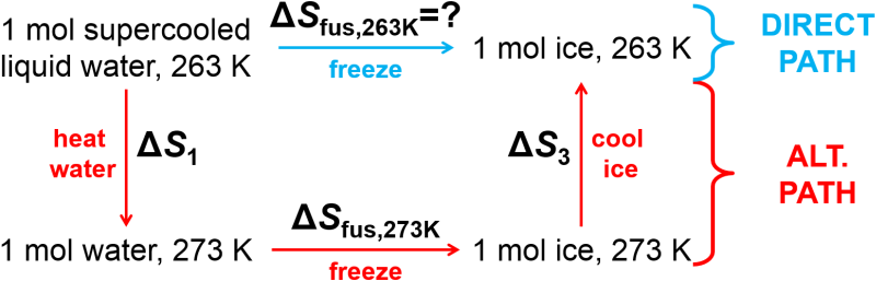
Fig. 3.4 Alternate path entropy calculation for freezing of supercooled water. All steps are reversible.
First, step 1 for the heating of water.
Second, step 2 for the equilibrium freezing of water at 273 K.
Third, step 3 for the cooling of ice.
We can add these all together to determine the change in entropy of the system.
Here we obtained a negative value for the change in entropy of the system for this irreversible (spontaneous) process. This would be expected for liquid water that freezes to solid water since there should be fewer configurations possible for solid vs liquid water. At the same time, since the process is irreversible, and all irreversible processes have \(\Delta S_\textrm{univ}>0\), we can also expect that \(\Delta S_\textrm{surr}>0\) by a sufficient amount that the overall entropy change of the universe is positive.
Now, how do we calculate the entropy change of the surroundings? This part is a little weird. We don’t have the details about what constitutes the surroundings in this problem. These details are often not provided. However, we did see in the problem statement that the process occurs at a constant temperature of 263 K, as if there were a very large thermal bath around the system. The bath is so large that when a little heat is transferred to it when the system freezes (that is exothermic, right?) the temperature of the bath will not change. The real process described in this problem is irreversible, but the alternative reversible path for the surroundings is just the slow addition of heat. It appears as if we can treat the surroundings reversibly, but that is just a consequence of the reversible alternative path for the surroundings being a very slow version of the real path.
Ok, let’s calculate the entropy change of the surroundings, now. We will use the relationship that heat lost by the system is the same as heat gained by the surroundings, or that \(q_\textrm{surr}=-q_\textrm{sys}\). Since this is a constant pressure process, it is also true that \(q_\textrm{sys}=\Delta H_\textrm{fus,263 K}\). In Section 2.5 we used an alternate path approach to determine for supercooled water that \(\Delta H_\textrm{fus,263 K}=-5640 \textrm{ J/mol}\), which saves us a little effort, here.
Lastly, we can calculate the change in entropy of the unvierse as
As expected, the positive entropy change of the surroundings more than compensated for the negative entropy change of the surroundings in order to make the overall entropy change of the universe positive.
3.5.1. Irreversible Entropy Calculations for an Ideal Gas
We just viewed example entropy calculations for a number of reversible ideal gas processes, and we will now turn our attention to irreversible ideal gas processes (see also Section 2.10 for a review of ideal gas processes covered so far). The second law states that entropy calculations for irreversible processes with ideal gases, or any other substances, must be performed along a reversible path. While many reversible alternative paths are possible for ideal gas processes, it turns out that we can come up with a single alternative path that works for them all, which is convenient.
The universal procedure is as follows.
First, calculate the initial and final states. This was reviewed in Section 2.10.
Second, construct an alternate path consisting of a reversible constant volume heating/cooling step and a reversible constant temperature expansion/compression step. Note that we have already calculated, above, the entropy change for these processes.
How can we be certain that two steps are sufficient and can be applied to all possible processes?
Consider the following process which goes from any valid combination of pressure, volume, and temperature to any other valid combination of pressure, volume, and temperature. (Valid here refers to the fact that the ideal gas law \(PV=nRT\) must still be obeyed.)
We can divide this arbitrary process into two reversible steps as shown, below. The first step in the alternative path is reversible constant volume heating/cooling to the final temperature \(T_2\) and the second step is a reversible constant temperature expansion/compression to the final volume \(V_2\). If at the end of the alternate path the temperature and volume match the final state of the system, then the pressure must, as well. Finally we can calculate the entropy change for the individual steps to determine the overall entropy change, using \(\Delta S_\textrm{sys}=\Delta S_1 + \Delta S_2\). (Note that this procedure works just as well if performing the constant temperature step first and the constant volume step second.)
We already calculated in our reversible ideal gas processes examples, above. Here are those results, shown again.
Here are a couple of notes on this procedure before doing some example problems.
There are sometimes irreversible ideal gas processes where only two variables change. In those cases, one of the two constant volume / constant temperature steps may be sufficient, and in that case the other step will return an entropy change of zero.
There are other possible reversible alternate paths that are valid.
We will discuss entropy of mixing, soon, which is a special case.
Example 6 (irreversible adiabatic compression). Calculate \(\Delta S_\textrm{sys}\), \(\Delta S_\textrm{surr}\), and \(\Delta S_\textrm{univ}\) when \(n\) moles of ideal gas at initial state \(P_1\), \(T_1\) are compressed adiabatically and irreversibly by a constant external pressure of \(2P_1\) until the system pressure matches the external pressure.
Part 1: Find the final state and be sure to use the real path. This uses skills from Irreversible Adiabatic Process but I have included it here to reinforce those earlier lessons. The new entropy calculation will start with part 2, below.
Here the pressure jumps suddenly up to twice the initial pressure, so we will use that as the constant external pressure. See also Principle of Maximum Work.
We can use energy and work terms, both expressed in terms of \(T_1\) and \(T_2\) to solve for the final temperature. Note that in the work expression, I factored out the \(nR\) terms and expanded the \(P_1\) term.
The above equation can be solved to find \(T_2=\dfrac{7}{5}T_1\) and we can use the ideal gas law to solve for \(V_2\) as shown below.
Part 2: Use our alternative reversible path approach for ideal gases to find the total entropy change for the system.
What about the entropy change of the surroundings and that of universe? Well, we must return to the real path in order to consider this. In that case, because this procedure was adiabatic, there was no heat transfer to the surroundings, so that \(dq=0\). We don’t need to even consider a reversible alternative path here to see that if there was no transfer of heat to the surroundings, then there was no entropy change for the surroundings. So \(\Delta S_\textrm{surr}=0\) and therefore \(\Delta S_\textrm{univ}=\Delta S_\textrm{sys} = 0.148nR\) which is a positive quantity as expected from the second law for all irreversible processes.
Example 7 (irreversible heating of an ideal gas at constant volume). A container of \(n\) moles of ideal gas in a rigid container and initially at \(P_1\), \(T_1\), and \(V_1\) is suddenly immersed into a hot bath at \(2T_1\), which heats to \(T_2=2T_1\) while maintaining a constant volume. Calculate \(\Delta S_\textrm{sys}\), \(\Delta S_\textrm{surr}\), and \(\Delta S_\textrm{univ}\).
We are already provided sufficient information to directly calculate \(\Delta S_\textrm{sys}\).
Since volume was held constant, here, it was not necessary to construct our alternate path to have two steps. We could have formally stated at single reversible alternate path with gradual heating at constant volume and then skipped the constant temperature step. However, it is convenient to have a universal solution in hand and we can see that it merely caused one term to be zero, so there was no harm done.
This time, heat was transferred between the system and surroundings along the real path of the process, so there will be an entropy change for the surroundings. When the temperature of the system jumped suddenly to the final temperature \(2T_1\), it is as if there was a very large thermal bath with temperature \(2T_1\). In that case we can figure out how much heat was lost by the surroundings at that temperature to figure out the entropy change. We can expect there to be a negative entropy change for the surroundings but that its magnitude should be smaller than that of the entropy change of the system so that the overall entropy change of the universe is positive for this system, since the second law says that is always true for irreversible processes. Let’s check.
Lastly, we can caclulate the entropy change of the universe, which we will see is positive, as expected.
What about a constant pressure reversible compression/expansion step for reversible paths?
Here is a lingering thought about reversible paths. We used a constant volume reversible step and a constant temperature reversible step to allow us to calculate any ideal gas path. Could use a constant pressure reversible step as part of an alternative reversible path?
In short, the answer is yes. Read below to see it worked out in general and for a specific case.
Let’s consider a reversible alternate path that uses a constant pressure compression/expansion in its first step, as shown generically, below, when going from initial state \((P_1,V_1,T_1)\) to \((P_2,V_2,T_2)\).
We can calculate the entropy change for the constant pressure step just fine from knowledge of the initial and final temperatures, as shown, below.
In the second step of the reversible alternate path, at constant temperature, we get the following.
Let’s return to the example problem above (\(n\) moles of ideal gas at initial state \(P_1\), \(T_1\) are suddenly compressed adiabatically and irreversibly to a final internal pressure of \(2P_1\), where we found \(T_2 = \frac{7}{5}T_1\)). In this case constant pressure step would give
and the temperatue step would give the following
for a total entropy change of
As expected, we obtain the same answer (\(0.148 nR\)) using a reversible alternate path consisting of constant pressure and constant pressure steps as we had obtained with a reversible alternate path consisting of constant volume and constant temperature steps.
3.5.2. Entropy of Mixing
The entropy of mixing is a sort of special problem that gets its own subsection. \(n\) moles of each of Ar and Xe at pressure \(P\) and temperature \(T\) are in adjacent containers of the same volume. The barrier between the two gases is removed, and the two gases mix. What is the entropy change of the system after it reaches equilibrium?
This problem may seem confusing at first. Removing a barrier to mix the gases will be an irreversible process so we can expect that the entropy change of the universe is positive. As with other irreversible processes, we want to find an alternative path between the initial and final states so we can calculate \(\Delta S_\textrm{sys}\). In particular, we can reversibly and isothermally expand each gas separately to reach the final volume and then by asserting that the inner barrier consists of a pair of semipermeable membranes we can allow the two containers to be combined. The part about the semipermeable membranes is a little goofy as a thought experiment, but it does get the job done. This reversible alternative path is shown in Fig. 3.5, below.
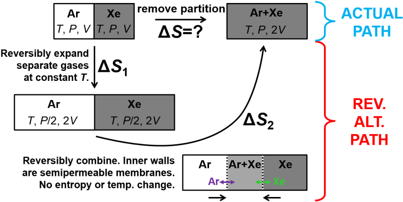
Fig. 3.5 Entropy of mixing. (Top) Removal of a partition in a box allows two gases to irreversibly mix. (Bottom) Reversible alternate path in which each gas is reversibly expanded to the final volume at a constant temperature and then the boxes are superposed by means of hypothetical semipermeable membranes that each transmit one of the gases but not the other.
Ok, using the slightly goofy alternate path with reversible steps, above, we can calculate the change in entropy. In particular, we just need to consider the reversible isothermal expansion step where heat is transferred to the system, and otherwise the gases would cool. As shown in Fig. 3.5, no heat is transferred during the combination step, so entropy does not change there even though the surroundings has to do some work to push the two boxes together. (Technically, all the entropy change occurs in the expansion steps not the mixing step so one could consider that entropy of mixing is a bit of a misnomer.)
Along the alternate path, each separate gas is maintained at a constant temperature. From the first law for an ideal gas (we are assuming ideal gases here), this means that \(q=-w\).
By symmetry in this problem, the entropy change of Xenon is the same.
From this, we can calcualte the total entropy change for the system as being
Now, what about the entropy of the surroundings and universe? Well, in the real path, there is no heat transferred to or from the surroundings, so the entropy change of the surrounings is zero, and we can see that \(\Delta S_\textrm{univ}=\Delta S_\textrm{sys} = 11.5n\dfrac{\textrm{J}}{\textrm{K mol}}\).
3.5.3. Summary of Entropy Calculation Results
We took a deep dive into entropy calculations for heating, phase changes, expansion, and both reversible and irreversible processes. Here is a summary of many of those results.
Process |
Result |
|---|---|
General reversible process |
\(\Delta S_\textrm{univ}=0\) and \(\Delta S_\textrm{surr}=-\Delta S_\textrm{sys}\) |
General irreversible process |
\(\Delta S_\textrm{univ}>0\) |
Reversible phase change |
\(\Delta S_\textrm{sys} = \dfrac{n\Delta H^\circ}{T}\) |
Reversible heating/cooling (constant heat capacity) |
\(\Delta S_\textrm{sys} = n\overline{C}\ln\dfrac{T_2}{T_1}\) |
Reversible constant volume heating/cooling of ideal gas |
\(\Delta S_\textrm{sys} = n\overline{C}_V \ln\dfrac{T_2}{T_1}\) |
Reversible constant temperature compression/expansion of ideal gas |
\(\Delta S_\textrm{sys} = nR \ln\dfrac{V_2}{V_1}\) |
Reversible constant pressure heating/cooling of ideal gas |
\(\Delta S_\textrm{sys} = n\overline{C}_P \ln\dfrac{T_2}{T_1}\) |
Reversible adiabatic process |
\(\Delta S_\textrm{sys} = 0\) |
3.6. Third Law and Absolute Entropy
Planck’s statement of the third law of the thermodynamics is as follows.
The entropy of a pure, perfect crystalline substance at 0 K is zero.
The third law provides us with a convenient reference point for entropy as an absolute quantity. Remember that internal energy and enthalpy do not generally have a good reference point and we saw in Enthalpy of Formation that scientists have decided to define the enthalpy of formation as zero for pure elemental substances in their stablest forms at 298 K, 1 bar. The notation of enthalpy of formation as having a \(\Delta\) symbol in the front helps to convey this idea, such as for \(\Delta_f H^\circ_{\ce{H2O}}\). In contrast, entropy has an absolute reference point where the entropy of a pure, perfect crystalline solid at 0 K is 0.
We can also relate entropy to Boltzmann’s entropy equation which related entropy to the number of available configurations as \(S = k_\textrm{B}\ln W\). A pure, perfect crystalline solid at 0 K has only one possible configuration, and with \(W=1\) we can expect that \(S=0\) since the natural log of 1 is 0.
With an absolute reference point, now, and with values for the temperature-dependent heat capacity over all temperature ranges of interest and enthalpies of phase transitions, we can calculate the absolute entropy of a substance by integration of the temperature-dependent heat capacity and addition of the entropy of phase transitions (see equation, above). Here we are assuming that the substance was a pure, perfect crystalline solid at 0 K and we will seek to find the absolute entropy of a substance in the gas phase. The same procedure could be adapted to find the absolute entropy as a solid, liquid, or gas at any desired temperature such as is plotted for \(\ce{Cl2}\) in Fig. 3.6.
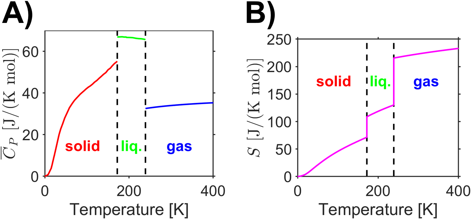
Fig. 3.6 Data for chlorine’s A) heat capacity vs temperature and B) absolute entropy vs temperature. (Data from [15], [16], and [18]) source
Now that we have introduced the absolute reference for entropy, we are in a position to discuss the fact that absolute entropy is actually tabulated for many compounds. We can use these tabulated absolute entropy values to calculate entropy changes for substances as you did with enthalpy. Let’s do an example.
Example 1: One of the most important industrial chemical process to human kind is the Haber-Bosch synthesis of ammonia for fertilizer from nitrogen and hydrogen. Calculate the entropy change per mole of ammonia formed from nitrogen gas and hydrogen gas at 298 K, 1 atm, all in the gas phase. The entropy of the relevant reagents is \(S_{\ce{N2}}=191.2 \frac{\textrm{J}}{\textrm{K mol}}\), \(S_{\ce{H2}}=130.7 \frac{\textrm{J}}{\textrm{K mol}}\), and \(S_{\ce{NH3}}=192.5 \frac{\textrm{J}}{\textrm{K mol}}\).
We can calculate the entropy changes similarly to how we calculated enthalpy changes with Eq. (2.2) using Eq. (3.4), below.
The balanced chemical reaction for the synthesis of ammonia is
and our equation for the entropy change is
Notice that the above is for one mole of reaction as written, however the question asked what is the entropy change for one mole of ammonia which is half of the above value. Beyond that, note that the change in entropy for the reaction is negative (for the system). This reflects the fact that the number of gas phase particles decreased in the reaction from 4 moles of reactants to 2 moles of product, and that there is a corresponding loss of translational entropy. The second law must still hold, however, and we can infer that the overall entropy change of the universe must be greater than (or equal to) zero based on some positive entropy change in the surroundings.
3.7. Heat Engines and the Carnot Cycle
Scientists and engineers of the industrial revolution were very interested in how to convert heat to work and the limits of efficiency in doing so. We saw that the reversible expansion of a gas (due to heating) maximized the amount of work attainable, but that was for a noncyclical process. We will soon revisit this point with cyclical processes like in a steam engine. It was precisely the analysis of cyclical processes like heat engines that led to the second law which generalizes in profound ways to a huge range of problems and disciplines from automobile combustion engines to refrigerators to the weather. In chemistry, the second law very importantly allows us to predict whether a process is spontaneous or not, that is, whether a process can occur without the input of external energy.
3.7.1. Overview of Heat Engines
At its core, a heat engine is a device which uses a cyclic process to convert thermal energy into mechanical work (Fig. 3.7). In each cycle, some heat \(|q_\textrm{in}|\) is inputted to the working substance of the heat engine from a hot reservoir at temperature \(T_\textrm{hot}\), some heat \(|q_\textrm{out}|\) is exhausted to cold reservoir at temperature \(T_\textrm{cold}\), and some net work \(|w_\textrm{out}|\) is done on the surroundings. Note that the input and output energies are equal, as required by the first law, with \(|q_\textrm{in}|=|q_\textrm{out}|+|w_\textrm{out}|\). Later, we will more carefully define the signs of these quantities, but we can use the absolute values for the time being.
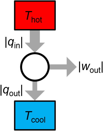
Fig. 3.7 Overview of a heat engine.
A pressure-volume heat engine for a gas, shown generically in Fig. 3.8), uses thermal energy from a hot reservoir to expand the gas, and exhausts thermal energy to a cool reservoir during compression. The system does work on the surroundings during expansion, and during compression, the surroundings does work on the system, but of a smaller magnitude, such that the area within the cycle is the net work done. The whole process can be repeated cyclically as in a combustion engine while transfering some of the thermal energy from the hot reservoir to useful work on the surorundings, such as in a combustion engine.
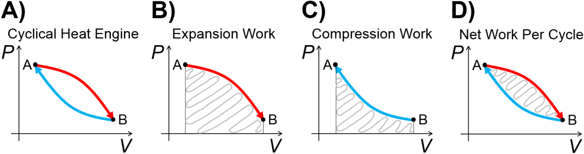
Fig. 3.8 Graphical overview of a pressure-volume heat engine. A) Basic cyclical design. B) Expansion step. C) Compression step. D) Net work done per cycle.
3.7.2. Carnot Cycle
Now, how do we construct an efficient heat engine? First of all, we need to use reversible steps since we saw prevoiusly that reversible expansion allows the maximum amount of work to be done by the system on the surroundings and that reversible compression required the minimum possible work to be done by the surroundings on the system. Out of convenience, we will use an ideal gas for the pressure-volume expansions. Second, reversible isothermal and adiabatic paths will turn out to be particularly simple for calculations, and we can use a pair of reversible isothermal and reversible adiabatic paths to trace out a nonzero amount of net work per cycle. This heat engine design is called the Carnot cycle (Fig. 3.9), an important theoretical development of French engineer Nicolas (Sadi) Carnot. We will analyze the Carnot cycle in some detail and then generalize the result to other thermal cycles.
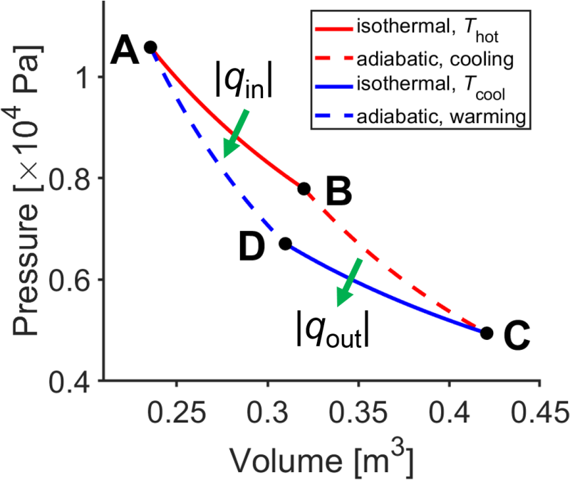
Fig. 3.9 Carnot cycle. source
Take a look at the design of the Carnot cycle.
Question: Why is the Carnot cycle designed with two isothermal steps and two adiabatic steps? Well, it turns out that on a \(PV\) plot, isothermal curves don’t cross each other and adiabatic curves don’t cross each other, but isothermal curves do cross adiabatic curves. Let’s prove that these things are true.
In the Carnot cycle, there are two reversible isothermal steps at different temperatures. Could these isotherms cross? Let’s use some mathematical reasoning to show that this is impossible. If two isotherms at two different temperatures, \(T_1\) and \(T_2\), did cross at the point \((P_\textrm{c},V_\textrm{c})\), they would have the same volume and pressure at the crossing point. This would mean that \(P_\textrm{c}=\dfrac{nRT_1}{V_\textrm{c}}=\dfrac{nRT_2}{V_\textrm{c}}\) which isn’t possible unless the temperatures are the same. Therefore, two isotherms at different temperatures cannot cross.
To connect the reversible isothermal steps in the Carnot cycle we will use two reversible adiabatic steps. Let’s show that the two adiabatic curves do not cross, this time using a graphical approach (Fig. 3.10). Reversible adiabatic processes all have \(\Delta S=0\), so both of the hypothetical adiabats would have no entropy change. However, we would be able to connect the hypothetical crossing adiabats with a reversible constant pressure process that must have a nonzero entropy change (Table 3.1). This logic would lead to the incorrect conclusion that going around in a cycle would have a nonzero value for \(\Delta S_\textrm{cycle}\) which is impossible since entropy is a state function. Therefore, reversible adiabats cannot cross.
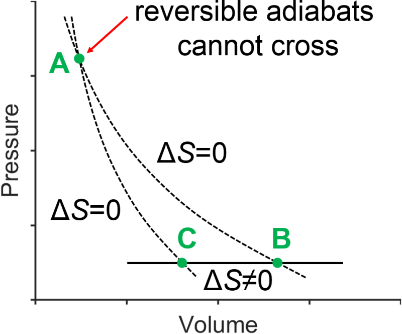
Fig. 3.10 Reversible adiabatic curves (dashed lines) cannot cross as shown in this impossible thermal cycle.
Next, let’s calculate the efficiency of the Carnot cycle (Fig. 3.9). Heat enters during step AB, exits during step CD, and in the process does some net work on the surroundings during steps BC and DA. We want to know how efficiently heat inputted into the system, \(q_\textrm{AB}\), is converted into work on the surroundings. We will define efficiency as follows.
We can look at a few relationships to help calculate this in terms of the input and output heats. First, recognize that work done on the system in one cycle is the negative of the work done on the surroundings in one cycle.
Since internal energy is a state function with \(\Delta U_\textrm{cycle,sys}=0\), it must be the case that
The two previous equations combine to give
Looking specifically at \(q_\textrm{cycle,sys}\), now we can see that
This can be plugged into our efficiency equation to yield the following.
Note that in the above equation, the term \(-\left| \frac{q_\textrm{CD}}{q_\textrm{AB}} \right|\) was used in order to avoid possible confusion about which term is positive and which is negative (note that \(q_\textrm{AB}\) is positive and \(q_\textrm{CD}\) is negative).
We can also relate the efficiency to the temperatures of the hot and cold isothermal steps of the Carnot cycle. For this, we will note that \(\Delta S_\textrm{cycle,sys}=0\) and that for the reversible adiabatic steps BC and DA, \(\Delta S_\textrm{BC}=\Delta S_\textrm{DA}=0\). From this, we can conclude that the entropy changes for the reversible isothermal steps must be equal and opposite so that they cancel out to zero for the overall cycle.
The entropy change for a reversible isothermal expansion/compression with an ideal gas is \(\Delta S_{\Delta T=0}=q/T\) so that the above equation becomes
The above can be rearranged to form
and then substituted back into our efficiency equation to give
This is an important result. We now see that there is a fundamental limit as to the efficiency of a reversible heat engine (the theoretically most efficient heat engine since it uses perfect, reversible steps) and we see that the efficiency is a simple function of the temperature difference between the hot and cold reservoirs. The smaller the ratio \(T_\textrm{cold}/T_\textrm{hot}\), the higher the efficiency and vice versa. In principle, with access to an infinitely hot reservoir for \(T_\textrm{hot}\) or with access to a cold reservoir near 0 K, we can get nearly perfect efficiency.
Importantly, our result for the Carnot cycle efficiency can generalize as the limit for any thermal cycle and for any working substance, not just a Carnot cycle using an ideal gas. Let’s consider the following logic in support of this conclusion. First, a reversible heat engine will be more efficient than an irreversible one. This is basically the principle of maximum work applied to reversible and irreversible processes. Second, all reversible heat engines for given hot and cold temperature baths have the same efficiency. This is because we can ‘decompose’ any arbitrary reversible process into a series of Carnot cycles which all obey the same efficiency limitation. In Fig. 3.11, an arbitrary \(PV\) cycle is approximated as a series of isothermal-adiabatic segments (the crisscross lines) which are a linear combination of Carnot cycles and are still subject to the efficiency limitation; by using a very large number of isothermal-adiabatic segments, the \(PV\) cycle could be approximated arbitrarily well. Third, all substances have the same theoretical maximum efficieny. Since the efficiency with an ideal gas already approaches 100%, an even higher efficiency would lead to a perpetual motion machine. So, regardless of the choice of thermal cycle and working substance, the Carnot cycle generalizes to telling us the limit of efficiency of converting heat into work with a simple equation (Eq. (3.5)).
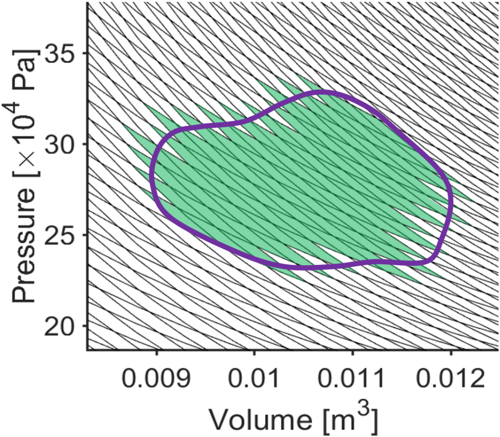
Fig. 3.11 Any thermal cycle (purple) can be approximated arbitrarily well as a series of Carnot cycles (green shaded region). The steeper black curves are adiabats and the less steep black curves are isotherms.
Practice Carnot cycle efficiency calculation.
Questions:
Assume a power plant has a ‘boiler’ with a temperature of 800 K and a condenser with a temperature of 500 K. What is the maximum achievable efficiency?
If 400 J of heat are absorbed from the hot reservoir (boilier) in one cycle for the power plant in problem 1, above, how much heat is exhausted to the cold reservoir per cycle? Assume the maximum theoretical efficiency is achieved.
Answers:
The maximum achievable efficiency is
The heat exhausted to the cold reservoir per cycle is
which we can solve to give \(q_\textrm{CD}=250 \textrm{ J}\).
Real combustion engines operate with some of the principles we are discussing for the idealized Carnot cycle heat engine. It will be instruction to examine how the work performed per cycle, \(w_\textrm{cycle}\) relates to the temperatures for the Carnot cycle.
First, let’s calculate work from all four steps starting with the isothermal steps AB and BC
and similarly
It turns out that the work in the two adiabatic steps BC and DA are equal and opposite.
We can put all four work terms together to get the work done per cycle as
Next, we need to relate the volumes to simplify \(w_\textrm{cycle}\) further. Because there is no entropy change during the reversible adiabatic steps BC and DA, we know the entropy change for the two isothermal steps must be equal and opposite (\(\Delta S_\textrm{AB} = -\Delta S_\textrm{CD}\)) so that the total entropy for going around the cycle is zero. We can also relate these nonzero entropy changes to volume for the reversible isothermal processes using our earlier result (Table 3.1) as
From this we see that
which we can substitute back in to our expression above for \(w_\textrm{cycle}\) to get
Our conclusion is that a larger compression ratio \(V_\textrm{B}/V_\textrm{A}\) and a larger temperature difference between the hot and cold baths leads to the largest magnitude work done per cycle. In the next section, we will see how that plays out with thermal cycles modeled after real combustion engines.
3.8. Beyond the Carnot Cycle
Let’s take a look at a few examples of other types of heat engines and thermal cycles besides the Carnot cycle. While we won’t be analyzing these quantitatively, the exercise can provide important insights.
3.8.1. Otto Cycle
The internal combustion engine used by most gasoline-powered cars operates approximately like that of the Otto Cycle (Fig. 3.12), named after German engineer Nicolaus Otto. Air and fuel (gasoline) are injected during A-B, compressed adiabatically and heated during B-C by the inertia of the engine (e.g., a fly wheel), ignited by a spark plug and combusted at constant volume during C-D, expanded adiabatically and cooled during D-E, further cooled at constant volume during E-B, and the combustion products are exhausted during B-A.
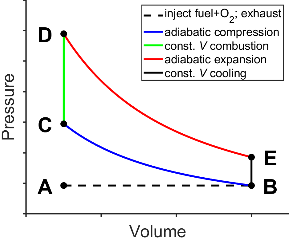
Fig. 3.12 Otto cycle. source
3.8.2. Diesel Cycle
Related to the Otto cycle is the Diesel cycle (Fig. 3.13), invented by German engineer Rudolf Diesel. Air is inputted into the system during A-B, compressed adiabatically and heated during B-C by the inertia of the engine (e.g., a fly wheel), injected into the cylinder during C-D which ignites as the piston moves (so the pressure is approximately constant), expanded adiabatically and cooled during D-E, further cooled at constant volume during E-B, and the combustion products are exhausted during B-A.
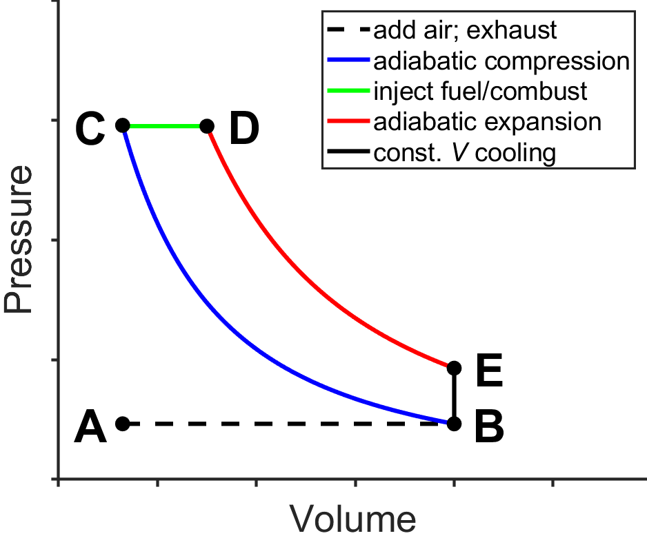
Fig. 3.13 Diesel cycle. source
For both the Otto and Diesel cycles, the compression stroke B-C leads to heating of the contents of the piston. In the case of the Otto cycle, the timing of ignition is controlled by a spark plug. This means that the compression stroke B-C in the Otto cycle cannot be so large as to reach a temperature where spontaneous ignitition is likely since this would lead to inconsistent timing that could cause the multiple pistons within an engine to fight one another and seriously damage the engine. For this reason, many automobile owners know to listen for uneven humming of a car’s engine (sometimes known as ‘knocking’). In the case of the Diesel cycle, however, only air is heated during the compression stroke B-C, and since there is no concern of premature ignition, the air can be heated to a much higher temperature by means of a large compression stroke. The injection of the fuel initiates combustion and doesn’t require the use of a spark plug. As a result of the higher compression ratio, the Diesel engine has an efficiency advantage in terms of a higher combustion temperature, although there are many practical considerations unrelated to the thermal cycles which also impact the overall efficiency of the two cycles.
Note that differences in the thermal cycles between the Otto cycle and the Diesel cycle are independent of the choice of fuel used in engines based on these cycles. Diesel fuel tends to be less volatile and more viscous than gasoline and the respective engines are carefully designed around these key properties of the fuels in terms of flash points, ability to lubricate parts, energy density, and so forth. In principle, the Otto and Diesel cycles could be operated with any fuel, but in practice I don’t recommend the experiment!
On a practical level, Diesel engines operate more efficiently (greater miles per gallon and miles per dollar), with less pollution, and for more miles before failure, than gasoline engines. Despite this, it is interesting to note that in the U.S., only some classes of vehicles routinely use Diesel engines, including freight trucks, ships, and trains–these vehicles are used in industries where efficiency and longevity are highly prioritized. Personal automobiles generally still run on gasoline in the U.S., with ~3% of new cars being Diesel, in contrast to the E.U. where ~20% of new cars are Diesel (data ~2022). Reasons for the lack of widespread adoption of Diesel engines in the U.S. may include the fact that Diesel engines are more expensive initially than gasoline engines, and that the U.S. imposes higher taxes on Diesel fuel than gasoline fuel (in many E.U. coutries it is the reverse). As of 2023, electric and hybrid cars have gained substantial ground, in both U.S. and E.U. markets, however, and appear poised to continue to gain market share.
3.8.3. Other Heat Engines
Drinking Bird Heat Engine. You have probably seen the drinking bird toy before. It turns out to illustrate a large number of chemical principles. The head gets wet from dipping the beak into water, which leads to evaporation and cools the head relative to the body. This sets up hot and cold reservoirs. The glass body of the bird contains a volatile liquid like dichloromethane which has a relatively low boiling temperature (~40 °C) and whose vapor pressure is quite sensitive to temperature. This means it is relatively easy for a small temperature change to expand gases to slosh liquid around in the bird to do mechanical work. In principle, if you were to try to run a drinking bird heat engine in an envirnoment where the air is saturated with water vapor, the drinking bird should stop operating.
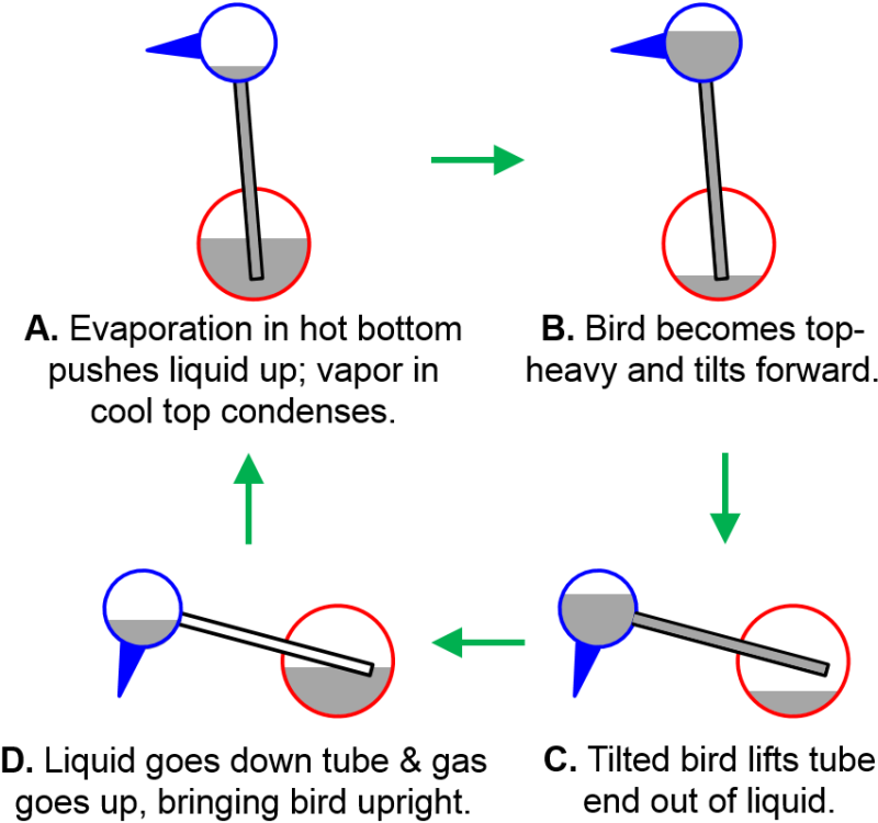
Fig. 3.14 Drinking bird heat engine.
3.9. Perpetual Motion Machines
The laws of thermodynamics are so well established that they have withstood multiple scientific revolutions. They were well in place before the atomic hypothesis was fully accepted, before quantum mechanics existed, and constitute one of the most highly tested ideas in all of science. In fact, if somebody tries to patent something that in which they claim an invention that violates the first or second laws of thermodynamics (by being a perpetual motion machine in some form) the US patent and trademark office won’t even consider the idea. In a sense, you could say that the laws of thermodynamics are also U.S. law.
3.9.1. Alternative Statements of the Second Law of Thermodynamics
The second law has fascinated scientists for almost two centuries. The law can be expressed in many ways that highlight specific aspects of the law or specific scenarios. Three of these statements are listed below, all in slightly modified and simplied forms.
Kelvin statement: It is impossible in a cyclic process to convert heat to work without also transferring some heat to a colder reservoir.* This aspect of the second law is also evident from examining the Eq. (3.5) which approaches 1 only in the limit of \(T_\textrm{cool}/T_\textrm{hot}\) approaching zero but isn’t experimentally realizable.
Clausius statement: It is impossible in a cyclic process to transfer heat from a cold reservoir to a hot reservoir without at the same time converting some work into heat.* Clausius’s statement is complementary to Kelvin’s statement, above, with a focus more on processes like those performed by an air conditioner (or heat pump).
Boltzmann statement: Nature tends to progress from less probable to more probable states.* Boltzmann’s statement encapsulates the second law very generally and elegantly, while at the same time managing to sound perfectly obvious.
Now, let’s take a look at some thermal cycles to see whether they are possible or whether they violate the laws of thermodynamics. Impossible thermal cycles or devices are sometimes referred to by the terms perpetual motion machine of the first kind, which refers to a violation of the first law of thermodynamics (e.g., outputing more energy than is input), or perpetual motion machines of the second kind, which refers to a violation of the second law of thermodynamics (e.g., energy is moved spontaneously from a cold to a hot reservoir).
Proposed Thermal Cycle 1
Question: A proposed reversible heat engine in each cycle performs 5 J of work on the surroundings, exhausts 2 J of energy to a low temperature bath, and absorbs 3 J of energy from a high temperature bath. Is the thermal cycle possible? If not, does it violate the first law or the second law?
Answer: This thermal cycle is impossible. It is a perpetual motion machine of the first kind since it violates the first law of thermodynamics. See the graphical illustration of the thermal cycle in Fig. 3.15, below, where 3 J of heat is inputted to the thermal cycle but 7 J are outputted (2 J to the low temperature reservoir and 5 J to do work on the surroundings).
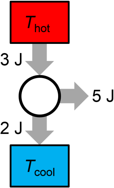
Fig. 3.15 Impossible thermal cycle.
Proposed Thermal Cycle 2
Question: A proposed reversible heat engine in each cycle performs 10 J of work on the surroundings, absorbs 20 J of heat from a high temperature bath, and exhausts 10 J of heat to a low temperature bath. Is the thermal cycle possible? If not, does it violate the first law or the second law?
Answer: The thermal cycle is possible. Neither the first or second laws are violated as shown in Fig. 3.16. Could you predict the value of \(T_\textrm{cold}/T_\textrm{hot}\) and the theoretical maximum efficiency for this thermal cycle?
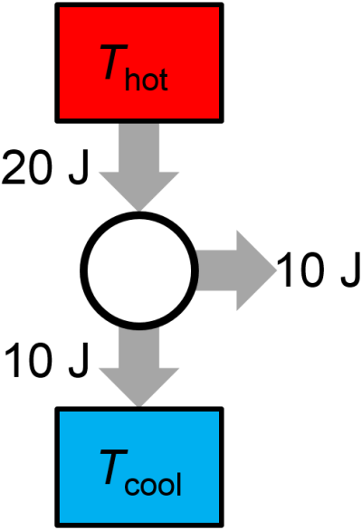
Fig. 3.16 Possible thermal cycle.
3.10. Additional Problems
(in progress, 1/17/2023)
Ideal gas thermal cycle.
Question: An ideal gas is taken through the thermal cycle A-B-C-A, shown below, where all steps are reversible. Answer the following about properties of the system.
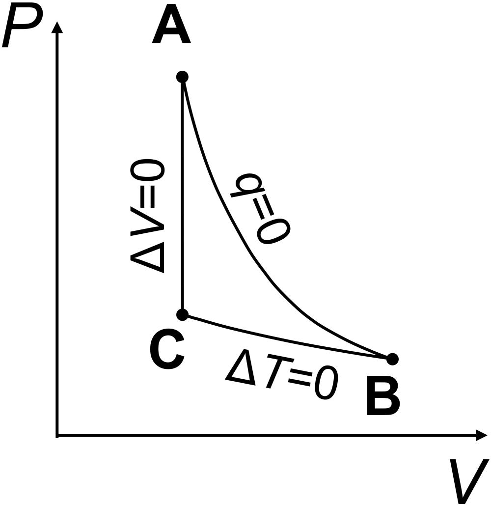
What is the sign of \(w_\textrm{cycle}\)?
What is the sign of \(q_\textrm{cycle}\)?
What is the sign of \(\Delta S_\textrm{cycle}\)?
What is the sign of \(\Delta S\) when going from point C to point A?
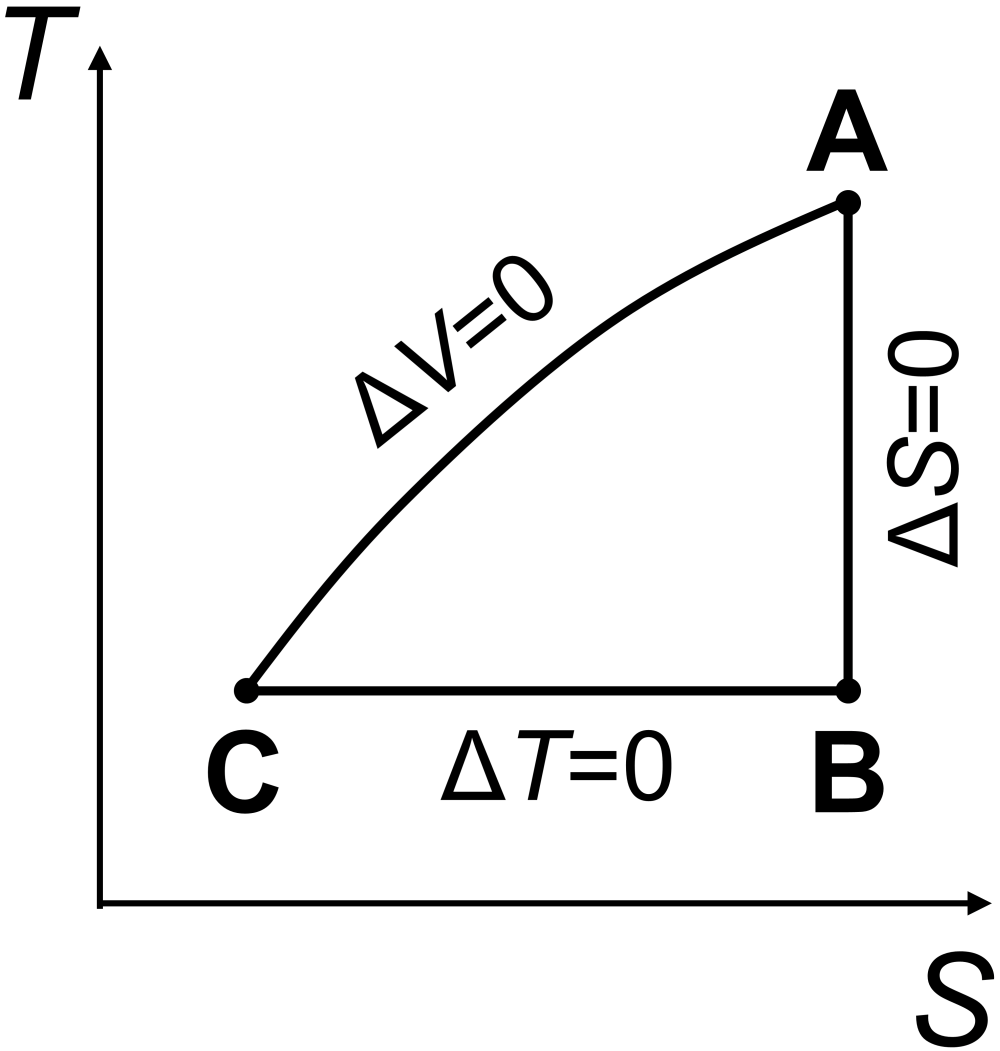
Make a sketch of the corresponding \(T\) vs \(S\) plot, and label the vertices.
Answer:
The total work on the system is negative, or \(w_\textrm{system}<0\). You can see this since the area under the \(PV\) curve for the expansion step (A to B, with negative work) is greater in magnitude than the area under the \(PV\) curve for the compression step (B to C, with positive work).
In one complete cycle, the change for any state function, such as \(\Delta U_\textrm{system}\), must be zero. The first law says \(\Delta U_\textrm{system}=q_\textrm{system}+w_\textrm{system}\). Since internal energy is a state function, for a cyclical process that ends up back where it started, we must have \(\Delta U_\textrm{system}=0\) so that \(q_\textrm{system}=-w_\textrm{system}\). Since we saw \(w_\textrm{system}<0\), we must have \(q_\textrm{system}>0\).
Since entropy is a state function, for a cyclical process that ends up back where it started, we must have \(\Delta S_\textrm{system}=0\).
The entropy change when going from C to A must be positive, \(\Delta S_\textrm{CA}>0\), as the system is heating up at constant volume.
See figure below.
Proposed Thermal Cycle 3
Question: A proposed reversible heat engine in each cycle performs 32 J of work, absorbs 32 J of energy from a high temperature bath, and releases no heat. Is the thermal cycle possible? If not, does it violate the first law or the second law?
Answer: This thermal cycle is impossible. It is a perpetual motion machine of the second kind since it violates the second law of thermodynamics. See the graphical illustration of the thermal cycle in Fig. 3.19, below, where the system is able to convert heat to work with 100% efficiency. This is a violation of the Kelvin statement of the second law.
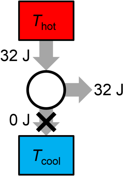
Fig. 3.19 Impossible thermal cycle.
Proposed Thermal Cycle 4
Question: For a proposed reversible heat pump (think more like an air conditioner than an engine), in each cycle 10 J of work are done on the engine, 30 J of heat are absorbed from a low temperature bath, and 20 J of heat are exhausted to a high temperature bath. Is the thermal cycle possible? If not, does it violate the first law or the second law?
Answer: The thermal cycle is impossible because it violates the first law of thermodynamics. As shown in Fig. 3.20, the heat pump inputs 40 J of energy from the combination of work (done by the surroundings) and heat extracted from the cold reservoir, but it only pumps 20 J of heat to the hot reservoir. These values don’t match.
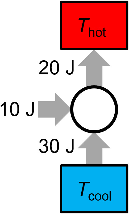
Fig. 3.20 Impossible thermal cycle.