2.1. Kinetic Theory of Gases

Let’s derive the fundamental result of the kinetic theory of gases which states that for an ideal gas, the gas’s kinetic energy is directly proportional to temperature.

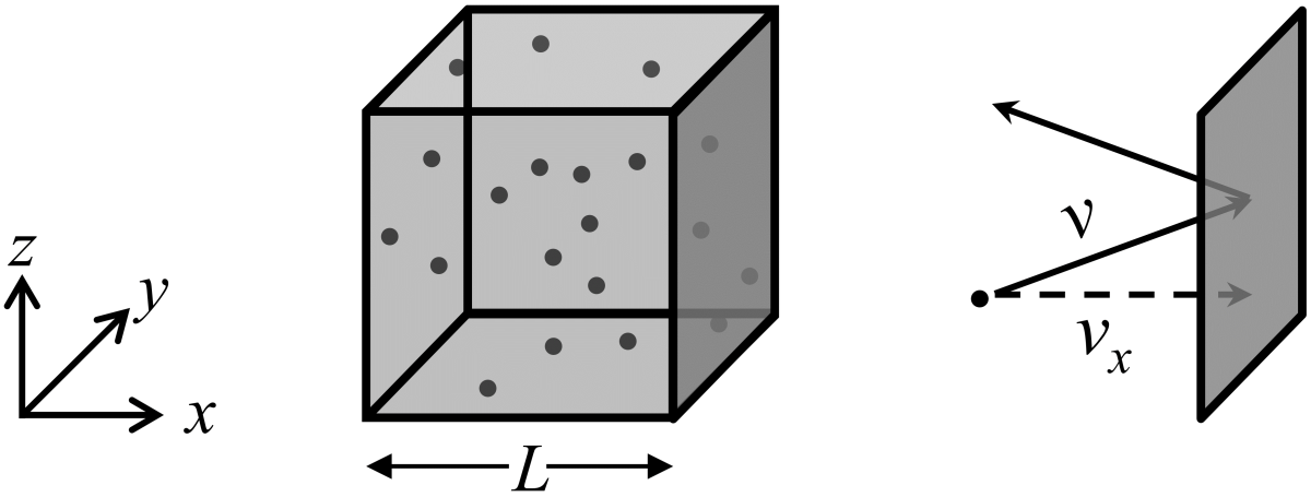
Fig. 2.12 System for kinetic theory of gas derivation.

Imagine a box shaped like a cube of edge length \(L\) that contains \(N\) ideal gas particles. The gas particles bounce around within the box, pushing on the box walls. We will use Newton’s laws to calculate the time-averaged pressure on the walls and then we can relate that pressure to temperature using the empirically-determined ideal gas law.

\[P = \frac{F}{A} = \frac{{nRT}}{V}\]

Before we dive into the math, let’s think a bit about the system. First, let’s assume that the particles are distributed randomly and travel with a random distribution of directions. From this we can expect that the time-averaged pressure is the same on all walls so it doesn’t matter which one we choose. Second, ideal gas particles are infinitesimally small and don’t collide with each other but do collide perfectly elastically (with no loss of kinetic energy) with the walls of the box. Third, we will calculate the force applied to one wall (perpendicular to the \(x\)-axis) and therefore we will work initially with the projection of the speed of a particle along the \(x\)-direction.

You probably remember Newton’s second law as \(F=ma\) for relating force \(F\) to mass \(m\) times acceleration \(a\), but we can also write it as the time derivative of momentum \(p=mv\) using \(F=dp/dt=d(mv)/dt=m(dv/dt)=ma\). With this, we can calculate the time-averaged force on the x-wall for one molecule, as indicted by the subscript \(x,\textrm{mol}\).

\[F_{x,\textrm{mol}} = \frac{dp_{x,\textrm{mol}}}{dt_{x,\textrm{mol}}} \approx \frac{\Delta p_{x,\textrm{mol}}}{\Delta t_{x,\textrm{mol}}} = \frac{2m{v_{x,\textrm{mol}}}}{2L/v_{x,\textrm{mol}}} = \frac{mv_{x,\textrm{mol}}^2}{L}\]

Note that the approximation, above, indicates the change in momentum over a long time period and not during a collision itself. This sometimes confuses students. Keep in mind that each colliding particle imparts a very brief force to the wall but that pressure results from the time-averaged average force applied by all the particles over a relatively long period of time. Once again, we are considering a long period of time, not the brief time during a collision.

The change in momentum along the \(x\)-direction is \(m\Delta v_{x,\textrm{mol}}=2mv_{x,\textrm{mol}}\) since a right-traveling particle with momentum \(mv_x\) will have a speed of \(-mv_x\) after a collision. The time between collisions with the \(x\)-face is the round trip distance along the \(x\)-direction divided by the speed along the \(x\)-direction, or \(\Delta t_{x,\textrm{mol}}=2L/v_{x,\textrm{mol}}\).

That was for one particle. Now let’s look at the time-averaged force on the \(x\)-wall due to all \(N\) particles. Note that the sum of all the square velocities of the \(N\) particles is the same as \(N\) times the average square velocities, and where the overline symbol indicates the average over all particles.

\[F_{x,\textrm{tot}} = \frac{m}{L}\left( {v_{x,1}^2 + v_{x,2}^2 + ...} \right) = \frac{m}{L}N\overline {v_x^2}\]

Putting force in terms of speed along the \(x\)-direction is a bit annoying, though. Let’s find a way to relate the speed along the \(x\)-direction to the actual speed of the particle. First, let’s use the Pythagorean theorem in three dimensions to see that the square speed equals the sum of the square speeds along each of the three cartesian coordinates. Second, let’s recognize that a system with particles traveling with a random (and uniform) distribution of directions means that the average square speeds along the \(x\), \(y\), or \(z\) directions must be equal. From these, we get the following:

\[\overline{v^2} = \overline{v_x^2} + \overline {v_y^2} + \overline{v_z^2} = 3\overline{v_x^2}\]

and therefore

\[\overline{v_x^2}=\frac{\overline{v^2}}{3}\]

Putting \(\overline{v_x^2}=\overline{v^2}/{3}\) into our equation for the time-averaged force along the \(x\)-direction for all \(N\) molecules we get:

\[F_{x,\textrm{tot}}=\frac{mN\overline{v^2}}{3L}\]

Next, we can use \(P=F/A=nRT/V\) to relate the force on the \(x\)-wall with area \(A\) to pressure from the ideal gas equation

\[P_x = \frac{F_{x,\textrm{total}}}{\textrm{A}} = \frac{mN\overline{v^2}}{3AL} = \frac{mN\overline{v^2}}{3V} = \frac{nRT}{V}\]

so that

\[\frac{1}{3}mN\overline {{v^2}} = nRT\]

Next, since \(N=N_\textrm{A}n\) (number of atoms equals Avogadro’s number \(N_\textrm{A}\) times number of moles) we can solve for the average square speed without any dependence on the number of moles. From this, we can see that the average square speed is linearly dependent on temperature.

\[\overline {{v^2}} = \frac{3RT}{mN_\textrm{A}}\]

Note that \(mN_\textrm{A}\) is the molar mass with units of mass per number of moles, and can be symbolized as \(M\). This gives us:

\[\overline{v^2}= \frac{3RT}{M}\]

At this point, we should take a closer look at the meaning of the average square speed since it is often confusing to students. The average square speed is the average of the square speeds of the particles but this is not the same as the square of the average speed. Here is an example to emphasize this point. Three particles with speeds \(4 \, \textrm{m/s}\), \(4 \, \textrm{m/s}\), and \(7 \, \textrm{m/s}\) would have an average speed of \(5 \, \textrm{m/s}\) and a squared average speed of \(25 \, \textrm{m}^2/\textrm{s}^2\). The square speeds would be \(16 \, \textrm{m}^2/\textrm{s}^2\), \(16 \, \textrm{m}^2/\textrm{s}^2\), and \(49 \, \textrm{m}^2/\textrm{s}^2\), giving an average square speed of \(27 \, \textrm{m}^2/\textrm{s}^2\). So if we want to get a quantity with units of \(\textrm{m/s}\) (like speed), we can take the square root of the average square speed that is also called the root-mean-square (RMS) speed. Although RMS speed will have units of speed, is not the same as the average speed, as we just saw.

\[v_\textrm{RMS} = \sqrt{\overline{v^2}} = \sqrt{\frac{3RT}{M}}\]

Next, we can relate kinetic energy to temperature. Since an ideal gas (assumed monotonic) can only have translational kinetic energy, its average kinetic energy \(\overline{\varepsilon}\) can be calculated using the average square speed.

\[\overline{\varepsilon}=\frac{1}{2}m\overline{v^2}=\frac{1}{2}m\frac{3RT}{mN_A}=\frac{3RT}{2N_A}\]

We can simplify a little further. Note that the ideal gas constant \(R\) when divided by Avogadro’s number \(N_\textrm{A}\) is known as Boltzmann’s constant \(k_\textrm{B}\), with \(R/N_\textrm{A}=k_\textrm{B}\). A simple way to think of it is that the gas constant \(R\) is for one mole of particles and Boltzmann’s constant \(k_\textrm{B}\) is the corresponding constant for one particle. We get the following:

\[\overline{\varepsilon}=\frac{3}{2}k_\textrm{B}T\]

These are cool results! Let’s take a minute to think about them. First, the mean square speed is proportional to temperature and inversely proportional to molar mass, so lighter or hotter particles will move fater than heavier or cooler ones. Second, for a given temperature, an ideal gas will have the same average kinetic energy regardless of the molar mass of the gas particle. Third, because the average kinetic energy of an ideal gas is strictly a function of temperature, it will cause changes in internal energy (and in enthalpy) of an ideal gas to be proportional only to temperature change, regardless of path, although the heat capacity will be path-dependent.

Finally, note that each spatial degree of freedom \((x,y,z)\) contributes \(k_\textrm{B}T/2\) to the overall kinetic energy. A system with more degrees of freedom (such as rotations or vibrations) adds additional terms of \(k_\textrm{B}T/2\) for each degree of freedom. This idea is known as the equipartition of energy theorem. It is primarily a topic of statistical mechanics, rather than thermodynamics, and won’t be addresed in detail here except briefly when discussing heat capacity.