6. Chemical Equilibrium
The word ‘equilibrium’ literally means a state of balance. We already discussed some aspects of equilibrium, with an emphasis on phase equilibrium, in Section 4, but let’s take a closer look now at four hallmarks of chemical equilibrium.
There is no net evidence of change.
The same final state is achieved regardless of the starting point.
There is a balance of forward and reverse processes.
There is no further potential for change.
The first two hallmarks of chemical equilibrium indicate that the equilibrium state is stable over time and that the same equilibrium state is reached regardless of the starting point (Fig. 6.1 A). The fact that the equilibrium state represents a balance of forward and reverse processes suggests that chemical processes continue to occur at the equilibrium state but that they have no net effect, which is a phenomenon known as dynamic equilibrium. Consider, for instance, the equilibrium state of a weak aqueous acid where ~25% of molecules are protonated at any one point in time. Although one would steadily measure on the ensemble level that ~25% of the acid molecules at any one time are protonated, individual molecules would in fact be transitioning back and forth between protonated and deprotonated states and would spend on average spend only ~25% of its time in the protonated state (Fig. 6.1). The equilibrium observed for a large ensemble of these fluctuating molecules would conceal the dynamics of individual molecules. The lack of potential for change for the equilibrium state indicates that the free energy of the system at equilibrium is minimized and that it is not possible to do any useful work, as we will see in the upcoming sections.
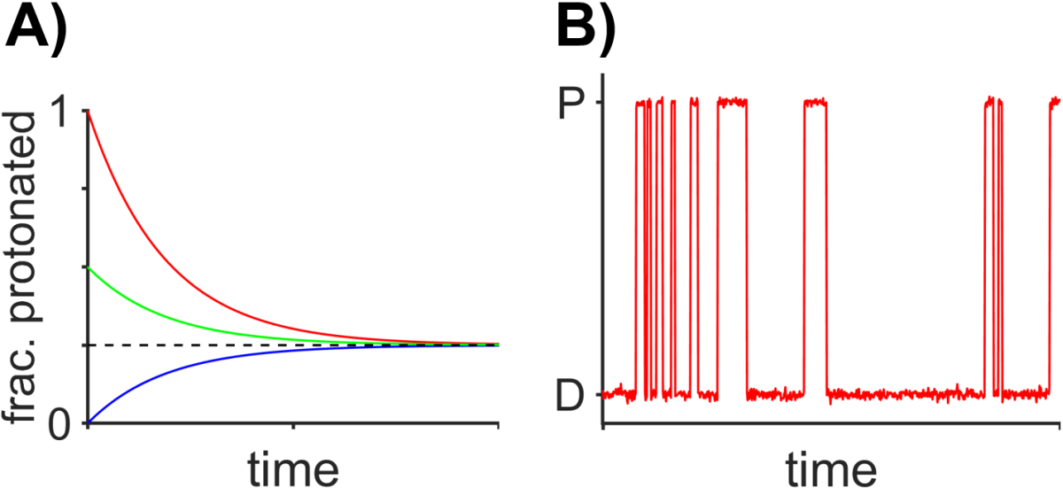
Fig. 6.1 Chemical equilibrium. A) Simulation of the fraction of molecules of a weak aqueous acid that attain the equilibrium state of 25% protonated regardless of the starting condition. B) Simulated dynamic equilibrium for a single molecule switching between a protonated state (P) and a deprotonated state (D). The molecule on average spends about ~25% of its time in the protonated state (P) and ~75% of its time in the unprotonated state. A large ensemble of molecules exhibiting this sort of random behavior will show, at any one time, ~25% of all molecules in the protonated state.
6.1. Law of Mass Action
Around the year 1870, Norwegian brothers-in-law and Cato Guldberg (a mathematician and chemist) and Peter Waage (a chemist) first formulated an idea that we now know as the law of mass action. The key insight of Guldberg and Waage was that the equilibrium state of chemical reactions resulted from the balance of concurrent forward and reverse reactions and they were able to obtain equilibrium constants from kinetic data for a series of experiments studying esterification reactions. The work of Guldberg and Waage build on ideas from many other chemists of the day, including a recent demonstration from Berthelot and Saint-Gilles that the reactions were proportional to reactant concentrations.
with reactants \(\textrm{A}_i\), products \(\textrm{B}_j\), and stoichiometric coefficients \(a_i\) and \(b_j\). The equilibrium constant \(K\) is given by
where the equilibrium partial pressures of the reactants are \(P_{\textrm{A}_i}\), the equilibrium partial pressures of the products are \(P_{\textrm{B}_j}\), and the reference pressure is by convention \(P_\textrm{ref}=1\textrm{ atm}\). Also recall that the product operator \(\prod\limits_{j}\) indicates multiplication of the indexed terms much like the sum operator \(\sum_j\) indicates addition of the indexed terms.
For solutions, the equilibrium constant would be
where the equilibrium concentrations of the reactants are \(C_{\textrm{A}_i}\), the equilibrium concentrations of the products are \(C_{\textrm{B}_j}\), and the reference concentration is by convention \(C_\textrm{ref}=1\textrm{ M}\).
Before doing a couple practice problems, let’s take a minute to think about several key points for these equilibrium expressions. By convention, we omit pure liquids or solids from mass action law (and equilibrium) expressions. Many people also omit \(P_{\textrm{ref}}\) and \(C_{\textrm{ref}}\) from the expressions, since it is cumbersome. If you want to do this, be very careful to input partial pressures with units of atm and concentrations with units of M (which cancel out with the reference pressure and concentration); equilibrium constants are unitless and mishandling of units can easily lead to errors.
Example 1: let’s practice writing out the law of mass action for the imaginary gas-phase reaction, written below.
We can write out our equilibrium expression from simple examination of the chemical reaction. All partial pressures are understood here as the equilibrium condition.
A more succinct equation for equilibrium constant. Let’s write out a more succinct general expression for the equilibrium constant. We will use the observation that the numerator terms for the products look a whole lot like the denominator terms from the reactants, and we can just use a convention where stoichiometric coefficients for products are positive, so that product terms go to the numerator, and where stoichiometric coefficients for reactants are negative, so that reactant terms go to the denominator. Accordingly, we will use one variable, \(\nu_j\), for the stoichiometric coefficient for component j, where the sign of the stoichiometric coefficient is negative for reactants and positive for products; we will use this same convention later in Chemical Kinetics.
Next, let’s do some practice problems that utilize the values of equilibrium constant.
Example 2: For the reaction \(\ce{3Al2Cl6(g)<=>2Al3Cl9(g)}\), the equilibrium partial pressure of \(\ce{Al2Cl6}\) is 0.75 atm and the equilibrium partial pressure of \(\ce{Al3Cl9}\) is 0.022 atm. What is the equilibrium constant?
Remember, generally speaking, that small equilibrium constants favor reactants, as is the case here, while large equilibrium constants favor products.
Example 3: Consider the decomposition of isopropanol into acetone and hydrogen, shown below, where the equilibrium constant is 0.52 at 155 °C. If 0.25 moles of isopropanol is placed into a 5 L vessel at 155 °C, a) what is the equilibrium partial pressure of acetone, and b) what fraction of isopropanol is dissociated at equilibrium? You may assume all gases here behave ideally.
First, let’s find the initial partial pressure of isopropanol using the ideal gas law; we already know that \(P_\textrm{AC,init}=P_{\ce{H2}\textrm{,init}}=0\).
Since we will plug the above into an equilibrium constant, where the reference pressure is 1 atm, we can convert units to obtain \(P_\textrm{IP,init}=1.76 \textrm{ atm}\).
Now, let’s see how things change at equilibrium. This is an example of an ICE problem (initial, change equilibrium), that most students will have studied in introductory chemistry courses. We already know the initial partial pressures, and we will let \(\Delta\) be equal to the partial pressure of \(\ce{H2}\) at equilibrium \(\left( P_{\ce{H2}\textrm{,eq}}\right)\); from there, we can determine how all species change with respect to \(\Delta\).
Now that we have all the equilibrium partial pressures in terms of the known initial partial pressures and \(\Delta\), we can evaluate the equilbrium expression and solve for \(\Delta\). Here, we will omit the reference pressure terms and units atm for convenience, remembering that all quantities will be in units of atm.
We can rewrite the above equation as a quadratic equation as
and then solve for \(\Delta\) with
which is \(\Delta = 0.731 \textrm{ atm}\) when using proper units. That gives the following values for the equilibrium partial pressures.
Finally, we can see that 42% of the isopropanol is dissociated.
6.2. Equilibrium in the Gas Phase
Let’s take a look at chemical equilibrium in the gas phase with the goal of relating the change in Gibbs free energy for an arbitrary reaction in the gas phase. It is an important result.
Let’s start by writing the change in molar partial Gibbs free energy for species i that starts at a partial pressure of one bar \(\left(P^\circ\right)\) and ends at an arbitrary actual partial pressure \(\left(P_i\right)\); this uses our equation for the change in Gibbs free energy when changing the pressure of a gas (Eq. (4.9)).
From this, we can obtain the partial molar Gibbs free energy for the species i.
In this case, for an arbitrary chemical reaction, we can write the following.
We can recognize that the first summation expression represents the change in molar Gibbs free energy for the reaction \(\left(\Delta\overline{G}_\textrm{rxn}^\circ\right)\) if conducted with all species at partial pressures of 1 bar. Next, we will use some logarithm algebra properties to simplify the second term so that the argument of the natural logarithm resembles our succinct equation for the equilibrium constant (Eq. (6.1)). Note, however, that the partial pressures are not necessarily at equilibrium, so we haven’t substituted for the equilibrium constant \(K\) here.
We can put these together to write
At equilibrium, we will have \(\Delta\overline{G}_\textrm{rxn}=0\) and all the partial pressures at their equilibrium state so that \(RT\ln\left(\prod\limits_{i} \left(\dfrac{P_i}{P^\circ}\right)^{\nu_i}\right) = RT\ln K\). This produces the familiar equation relating chemical equilibrium to change in Gibbs free energy, arguably, one of the most important equations in chemistry or biochemistry.
6.3. Equilibrium in the liquid phase
Equilibrium for solutions follows the same overall equation as for the gas phase, but will make use of the ideal solution equation (Eq. (5.5)) which states that
where partial molar Gibbs free energy \(\overline{G}_i\) is the same as chemical potential. Now, for solutions of species \(i\), we want to work with concentration \(c_i\), not mole fraction \(x_i\). For sufficiently dilute solutions (where the ratio of solution volume to total number of moles is approximately the same as the ratio of solvent volume to solvent number of moles) we can approximate as
where \(\overline{V}_\textrm{solv}\) is the volume per mole of the pure solvent. We can then replace mole fraction with concentrations in the ideal solution equation to get
Notice that the term \(\overline{G}_i^{\circ'}\left(\textrm{pure liquid}\right)\) includes the partial molar Gibbs free energy of the pure liquid \(i\), \(\overline{G}_i^{\circ'}\left(\textrm{pure liquid}\right)\) as well as the reference concentration term \(RT\ln \left( \overline{V}_\textrm{solv} \cdot 1\textrm{ M} \right)\).
As we did for the gas phase, let’s consider the arbitrary chemical reaction
and then write out the change in Gibbs free energy per mole of reaction. We will simplify the result a bit, as before, using logarithm properties.
Once again, at equilibrium, \(\Delta\overline{G}_\textrm{rxn} = 0\) and we can recognize that the product expression in the logarithm is just the equilibrium constant (Eq. (6.1)), giving us
where often it is simply written as \(\Delta\overline{G}_i^{\circ}\left(\textrm{pure liquid}\right)\) without explicit reference to the additional \(RT\ln \left( \overline{V}_\textrm{solv} \cdot 1\textrm{ M} \right)\) term.
6.4. Reaction Quotient
In the previous two sections, we considered the equilibrium state. Here, we will determine the change in Gibbs free energy for a reaction in an arbitrary state, equilibrium or otherwise. These results will be written out explicitly for the gas phase, but are almost identical in form for solutions.
Our expression for the gas phase equilibrium constant, \(\Delta\overline{G}_\textrm{rxn}^{\circ} = -RT\ln K\), is defined for equilibrium partial pressures. For a system that is not at equilibrium, we can define the reaction quotient \(Q\) as a quantity that looks almost idetnical to equilibrium constant except that the subscript ‘eq’ is absent from the expression (compare to Eq. (6.1)) indicating that the system may or may not be at equilibrium.
In this case we can write for the gas phase (and an almost identical equation for solutions) a modified form of (Eq. (6.2))
This equation indicates the change in Gibbs free energy for a reaction whether or not it is at equilibrium. As the system approaches equilibrium, \(Q\) approaches \(K\) and \(\Delta\overline{G}_\textrm{rxn}\) approaches zero, fully consistent with our result that \(\Delta\overline{G}_\textrm{rxn}^\circ = -RT\ln K\). It is a useful relationship since it shows that a system near to equilibrium yields a smaller magnitude of non-pressure-volume work (amount of Gibbs free energy) than a system that is farther from equilibrium.
It is important to keep in mind that it is still true that \(\Delta\overline{G}^\circ_\textrm{rxn}=-RT\ln K\) for gases. In this case we can write an equation that combines reaction quotient together with equilibrium constant
which can be simplified to
These results apply not only to gases, but also to solutions, by using concentration-based forms of reaction quotient and equilibrium constant and by using the solution standard Gibbs free energy \(\Delta\overline{G}_\textrm{rxn}^{\circ'}\) in place of the gas phase stanard Gibbs free energy \(\Delta\overline{G}_\textrm{rxn}^\circ\).
6.5. Temperature Dependence of Equilibrium
We can use the equilibrium statement for Gibbs free energy and relate to the temperature dependence of the equilibrium constant.
At equilibrium we have
and we can approximate that following
Combining the previous two equations gives
Next, approximating \(\Delta\overline{H}^\circ_\textrm{rxn}\) and \(\Delta\overline{S}^\circ_\textrm{rxn}\) as constant (over a sufficiently small range of temperatures) provides the following for temperatures \(T_1\) and \(T_2\)
where \(K_1\) and \(K_2\) are the equilibrium constants at temperatures \(T_1\) and \(T_2\), respectively. These two equations can be combined to give the van’t Hoff equation
The van’t Hoff equation is a convenient equation for relating echanges in the equilibrium constant to temperature and enthalpy change. Note that (Eq. (6.5)) resembles the Clausius-Clapeyron equation but applies to scenarios beyond phase equilibrium between a gas and a condensed phase.
6.6. Additional Example Problems
Let’s take a look at some ways in which chemical equilibrium can be informative for biologically-relevant experiments.
Ion Channels. Sophisticated instruments such as patch clamps can measure the electrical current transmitted by a single ion channel protein (Fig. 6.2). In these experiments, researchers observe bursts of current as the ion channel switches randomly between open and closed states. The fraction of time spent in the open (high-curent) vs closed (low-current) state can be used to estimate the open-closed switching equilibrium properties of the ion channel.
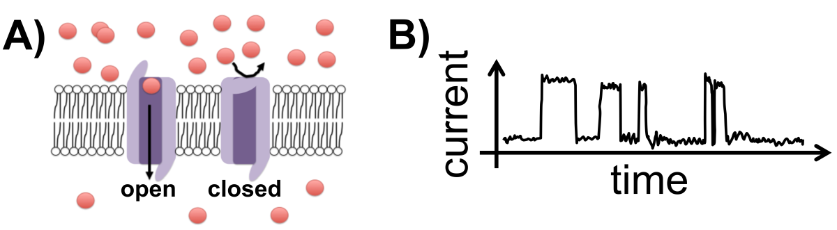
Fig. 6.2 Ion channels. A) Ion channels in a cell membrane in an open or closed state. B) Cartoon of current measurement from a single ion channel as it interconverts between an open (high-current) and a closed (low-current) state. (Ion channel image from Efazzari, under a CC-BY 4.0 license via Wikipedia.)
calculate equilibrium constant for ion channel switching
Question: What is the standard Gibbs free energy change describing the open/close state of the ion channel shown in (Fig. 6.2) for a temperature of \(T = 310 \textrm{ K}\)?
Answer:
The ion channel spends about 25% of its time open and about 75% closed. This information can be used to determine the equilibrium constant which, in turn allows calculation of
Amino Acid Partitioning and Protein Folding. The specific sequence of a protein determines the structure of the folded state. One key organizational principle for protein structure is that hydrophobic amino acids tend to aggregate to the hydrophobic core (interior) of the protein while hydrophilic amino acids tend to coat the surface of the protein. This simple structural principle is a key factor that helps proteins to fold rapidly (e.g., see “Levinthal’s paradox”). When simply analyizing the hydrophobicity sequence of amino acids in a protein, researchers, can often predict which stretches of amino acids are likely to exist in the core of the protein vs the surface. Such predictions rely on the measurement of the hydrophobicity of the amino acid building blocks, often using a simple equilibrium “partitioning” experiments.
One version of a partitioning experiment uses a mixture of octanol and water which separate like oil and vinegar in salad dressing. In that experiment, researchers would add an amino acid to the octanol-water mixture, agitate the sample and allow the amino acid to partition into the two layers of liquid (at equilibrium), and then sample the octanol and water phases to determine the concentration of the amino acid in each. From knowledge of these concentrations, the Gibbs free energy can be measured for the transfer of the amino acid from one liquid phase to another.
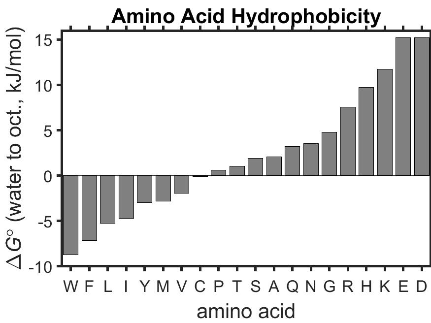
Fig. 6.3 Hydrophobicity of the 20 proteinogenic amino acids as measured by octanol-water partitioning. Data are replotted from Wimley et al. ([1]). source
Figure (Fig. 6.3) shows experimentally determined \(\Delta\overline{G}^\circ\) values for the transfer of amino acids from water to octanol. Not surprisingly, aromatic (hydrophobic) amino acids such as tryptophan (W) have a large negative value of \(\Delta\overline{G}^\circ\) since it is favorable for them to be transferred to a nonpolar environment like octanol, while charged, hydrophilic amino acids like glutamic acid (E) have a large positive value of \(\Delta\overline{G}^\circ\) since it is not favorable to be transferred from water to octanol. The \(\Delta\overline{G}^\circ\) values can be used to calculate equilibrium constants. Assuming \(T=310 \textrm{ K}\), we see that tryptophan has \(K=\exp\left(-\frac{\Delta\overline{G}^\circ}{RT}\right)=22\) (favors octanol) and that glutamic acid has \(K=0.0044\) (favors water).
calculate equilibrium constant for amino acid partitioning
Question: What is the equilibrium constant describing the partitioning of the amino acid cysteine (water to octanol) at \(T=310 \textrm{ K}\)? Use the data from figure (Fig. 6.3).
Answer:
Cysteine partitions about half to water and half to octanol.
An example of a hydrophobicity scan, performed by Kyte & Doolittle in 1982 ([2]), is shown for the protein lactate dehydrogenase (Fig. 6.4); large hydrophobic regions correspond to protein regions known from crystallography to exist in the core of the protein (purple lines) while large hydrophilic regions correspond to protein regions known to exist at the surface of the protein (green lines). More recent analysis has quantitatively determined how it is in fact contiguous stretches of hydrophobic amino acids that are required to form stable core protein domains ([3]).
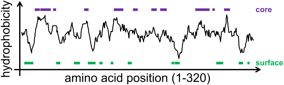
Fig. 6.4 Hydrophobicity scan of the enzyme lactate dehydrogenase showing that hydrophobic regions of the enzyme tend to associate with the core of the protein (as determined by x-ray crystallography) while hydrophilic regions of the enzyme associate with the surface of the protein. Data are replotted from Kyte & Doolittle ([2]).