5. Ideal Solutions and Colligative Properties
5.1. Raoult’s Law
Vapor pressure is the pressure of a vapor in equilibrium with a solid or liquid (Fig. 5.1 A) and where the vapor pressure can have a fairly strong dependence on temperature. For instance, the vapor pressure of water at 298 K is ~0.03 atm wheas the vapor pressure of water at 373 K is 1 atm. At a temperature above 373 K, water would have a vapor pressure greater than 1 atm. Now, in the case of a mixture of two liquids, A and B, we would expect to see two vapors in equilibrium with the liquid (Fig. 5.1 B). In this case, it would be reasonable to predict that the partial pressures of A or B would be larger for higher concentrations (or mole fractions) and for liquids that, in their pure form, have larger vapor pressures. These considerations are neatly summarized in an empirically-observed relationship known as Raoult’s Law.
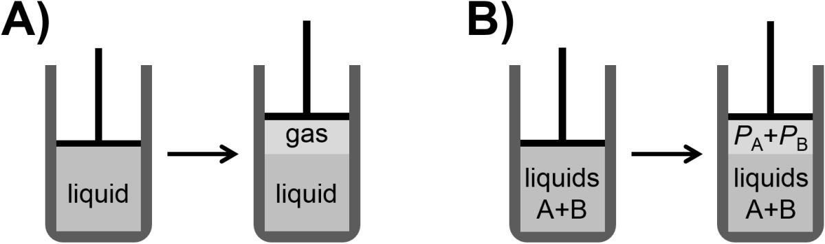
Fig. 5.1 Illustration of A) vapor pressure of vapor above a liquid and B) partial pressures of two species above a mixture of the two corresponding liquids.
Raoult’s law states that partial pressure above liquid \(i\) is proportional to the mole fraction of the liquid, \(x_i\), times the vapor pressure of the pure liquid \(P_i^*\) as shown in Eq. (5.1).
Some combinations of liquids are well described by Raoult’s law, but many deviations are also well-known. Fig. 5.2 shows examples with relatively large deviations in scenarios where solutes don’t resemble the solvent in terms of chemical groups (i.e., the solute-solute interactions differs prominently from solvent-solvent and/or solvent-solute interactions). So-called ‘positive deviations’ from Raoult’s law (e.g., Fig. 5.2 B) have higher pressures than predicted by Raoult’s law while ‘negative deviations’ from Raoult’s law (e.g., Fig. 5.2 C) have lower pressures than predicted by Raoult’s law. Even in these scenarios, however, note that for large values of mole fraction, Raoult’s law is obeyed quite well. Because of this, if is often stated that that for sufficiently dilute solutions Raoult’s law is valid for the solvent.
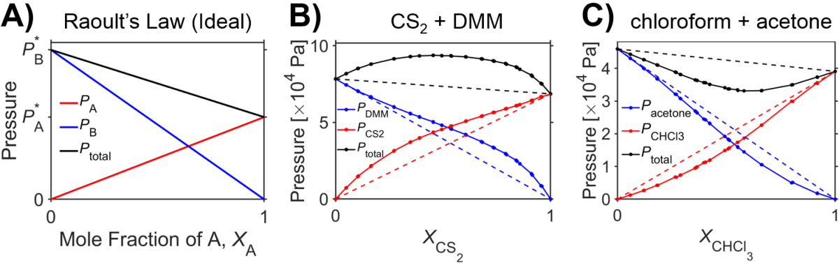
Fig. 5.2 Raoult’s Law. A) Ideal case for hypothetical liquids A and B. Measurements of partial pressure for B) a mixture of carbon disulfide and dimethoxymethane and C) a mixture of chloroform and acetone. Points indicate measured data and dashed lines indicate the predictions from Raoult’s law based on mole fraction and vapor pressures of the pure liquids. (Experimental data from [23].) source A source B source C
Example 1: What is the total vapor pressure of Jameson Irish Whiskey at 298 K? Assume Jameson is 40% ethanol and 60% water by mass and that it is well-described by Raoult’s law. The vapor pressures of ethanol and water at 298 K are 8000 Pa and 3200 Pa, respectively, and the molecular weights are 46 g/mol and 18 g/mol.
First, let’s find the mole fractions of ethanol and water for some general mass \(m\) (it won’t depend on this value).
Next, let’s apply Raoult’s law to find the total pressure.
As expected, the total pressure is part way between the vapor pressures of pure water and pure ethanol.
More practice with Raoult’s law.
Question: 0.5 g of a nonvolatile solute S is added to 18 g of \(\require{mhchem}\ce{H2O}\). The total vapor pressure decreases by 20 Pa and the vapor pressure of pure water is \(P_W^*=3200 \textrm{ Pa}\) at this temperature. What is the molecular weight of the solute? (Problem adapted from [17].)
Answer: The measured water vapor pressure is proportional to mole fraction of water in the solution, where the mole fraction of water will decrease as a function of the addition of solute S. We can therefore use the decrease in vapor pressure to determine the number of moles added to a solution and from knowledge of the mass of the solute, we can calculate the molecular weight of the solute.
Raoult’s law says that
which we can solve for \(n_\textrm{S}\) to give
Finally we can calculate molecular weight and substitute values, where 18 g of water corresponds to \(n_\textrm{W}=1 \textrm{ mol}\) to get
Interesting to know that measurement of vapor pressure can enable the calculation of molecular weight.
5.2. Chemical Potential
Let’s adapt the Gibbs free energy to explicitly include a term describing all the chemical components. Similar modifications may be made to the other energy state functions \(U\), \(H\), and \(A\), but we won’t be using these. Specifically, let’s consider the Gibbs free energy in the case where there are \(N\) total components, e.g., \(G(P,T,n_1, …n_\textrm{N})\), and where \(n_1\) is the number of moles of the first species, \(n_2\) is the number of moles of the second species, etc., and these components are present in the mixture but are not allowed to react. We can write out a general differential for this case.
From our prior knowledge of the differential of Gibbs free energy (Eq. (4.6)) we can recognize the first two partial derivatives as \(-S\) and \(V\), respectively, but the partial derivative term on the right is new. We will call this term the chemical potential and we will give it the variable \(\mu\) so that \(\mu_i\) is the chemical potential of the \(i^\textrm{th}\) component. We use the term chemical potential synonymously with partial molar Gibbs free energy \(\overline{G}_i\).
We can formulate a revised differential of Gibbs free energy that now includes multiple possible components.
There are different ways to think about chemical potential that may be helpful. One is that it is just the partial molar free energy of a specific component of a mixture. Another is that it is the free energy gained or lost when some number of moles of a component of your system is added. Another is to think of it analogously to other potential energy functions, such as gravitational potential energy. We will look at a few examples, soon, to help gain intuition for chemical potential, noting that we will mostly use it as a tool for fundamental derivations rather than calculating its explicit value.
Consider two phases \(\alpha\) and \(\beta\) that are in equilibrium with each other at constant \(P\) and \(T\) in an isolated container with \(n_\textrm{total}=n_\alpha+n_\beta\). (This section adapted from [17] and [22].) In that case our equation for the differential of Gibbs free energy Eq. (5.3) becomes
Now, if an infinitesimal perturbation \(dn\) converts some of phase \(\beta\) to \(\alpha\) (Fig. 5.3) then we would have \(dn_\beta=-dn\) and \(dn_\alpha=dn\) and our differential for Gibbs free energy would become
Since the system is at equilibrium (meaning \(dG=0\)) and an infinitesimal perturbation is not sufficient to disturb the equilibrium, then at equilibrium we must have the scenario that \(\mu_\alpha=\mu_\beta\). This is true for the phase transition case considered here and it is also true for the case of mass transport.
What if we consider a system not initially at equilibrium? For instance, if \(\mu_\beta>\mu_\alpha\) then our equation \(dG = \left( \mu_\alpha - \mu_\beta \right) dn\) would give \(dG<0\) (spontaneous) for \(\mu_\beta > \mu_\alpha\) and we would predict conversion of \(\beta\) to \(\alpha\). We will see later in our discussion of osmotic pressure that transport can occur spontaneously from regions of high chemical potential to regions of low chemical potential.
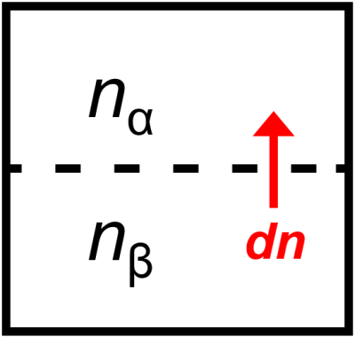
Fig. 5.3 Phases \(\alpha\) and \(\beta\) are in equilibrium with each other when an infinitesimal amount of \(\beta\), \(dn\) converts to \(\alpha\).
5.3. Ideal Solutions
An ideal solution consists of a solute dissolved in a solvent where the intermolecular forces are the same for solvent-solvent, solvent-solute, and solute-solute interactions. While this behavior is approximated in some dilute systems, we primarily introduced it here since it allows us to obtain a key relationship (the ‘ideal solution equation’) for studying Henry’s law and colligative properties.
Our general approach here is to use chemical potential and Raoult’s law to adapt our understanding of gas phase chemical equilibrium to a so-called ‘ideal solution’. We will consider a scenario where a vapor of species \(i\) is in equilibrium with a solution of \(i\). The chemical potential for vapor of species \(i\) at standard state pressure (\(P^\circ\) = 1 bar) is \(\mu_i^\circ(\textrm{vapor})\) and the chemical potential at partial pressure \(P_i\) is \(\mu_i(\textrm{vapor})\). Changing the pressure from standard state \(P^\circ\) to partial pressure \(P_i\) is given by
where the natural log term in the above equation resembles our earlier result (Eq. (4.9)) for a change in the Gibbs free energy of a gas upon change in pressure (but in this case also divided by number of moles). Now, for liquid and vapor phases in equilibrium, we have \(\mu_i(\textrm{solution})=\mu_i(\textrm{vapor})\) so that
Next, if we consider a special case of the above equation where species \(i\) is a pure liquid, indiated with a * symbol, that is in equilibrium with its vapor at the pure vapor pressure \(P_i^*\) then we obtain
The above two equations both contain the term \(\mu_i^\circ(\textrm{vapor})\). We can use that common term to combine the equation to get
Next, we can plug in Raoult’s law, \(P_i=x_iP_i^*\) to obtain the ideal solution equation
where Although real solutions may show prominent deviations from that of a hypothetical ideal solution, the ideal solution behavior is approximately observed for low solute concentrations and the simplicity of the ideal solution equation enables us to gain key insights into several interesting phenomena as we will see in the next sections.
5.4. Henry’s Law
Henry’s law is used to relate the pressure of a gas above a solution for species \(i\), \(P_i\), to the equilibrium mole fraction of the dissolved gas in the liquid using the equation \(P_i=k_i x_i\), where the Henry’s law constant \(k_i\) is valid for small mole fractions whether or not the solution behaves ideally. We can get a sense of this by re-examining some data used initially to illustrate deviations from Raoult’s law for a mixture of the liquids carbon disulfide and dimethoxymethane.
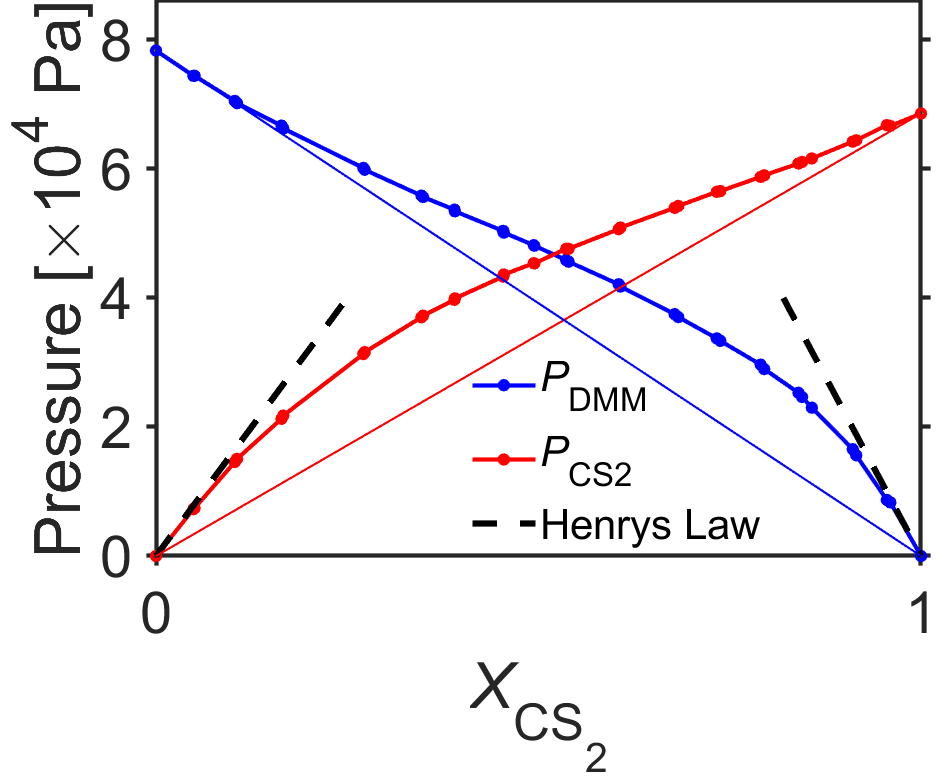
Fig. 5.4 Measurements of partial pressure for a mixture of carbon disulfide and dimethoxymethane illustrating Raoult’s law and Henry’s law for different regimes. Points indicate measured data (from [23]) and straight thin lines indicate the predictions of Raoult’s law. Henry’s law may be used as a line fit for sufficiently low mole fractions of solute (black dashed lines) although for nonideal solutions the slope is different than that of Raoult’s law. source
In Fig. 5.4 we can see that Raoult’s law is approximately valid for for high mole fractions, where the measured partial pressure asymptotically approaches the straight-line prediction from Raoult’s law. At the same time, for low mole fractions, the measured partial pressure approaches the Raoult’s law prediction at a nonzero angle. In this low mole fraction regime, instead of using Raoult’s law, we can do a linear approximation of the gas partial pressure using Henry’s law \(P_i = k_i x_i\). The Henry’s law constant \(k_i\) is the slope of the line and is a constant specified for a given gas dissolved in a specific solvent. While the data in Fig. 5.4 are plotted as a function of mole fraction of carbon disulfide, \(x_{CS_2}\) the mole fraction of dimethoxymethane is simply \(x_{DMM}=1-x_{CS_2}\) and can be seen to show similar behavior.
We can put Raoult’s law and Henry’s law together with these observations. An ideal solution is perfectly described by Raoult’s law, by definition, and in that case the Henry’s law constant would simply be equal to the vapor pressure of the pure liquid according to \(P_i=x_i P_i^*=k_i x_i\). For a dilute nonideal solution, partial pressure is still described well by Raoult’s law for high mole fraction, and for this reason it is often said that Raoult’s law is valid for the solvent. For a dilute nonideal solution, the partial pressure can be approximated at low mole fraction with a line using Henry’s law, and the counterpart statement is that Henry’s law is valid for the solute.
Let’s take a look at our ideal solution equation to rationalize Henry’s law.
For a gas ‘i’ in dissolved in a liquid, the chemical potentials will be equal.
Into the left side of the above equation substitute our ideal solution equation (Eq. (5.5))
and into the right side will use our earlier result for chemical potential when changing the pressure of an ideal gas (Eq. (5.4))
which gives us
Combining the natural log terms yields
We can solve the above partial pressure of the vapor \(P_i\) an obtain Henry’s law
where Henry’s law constant \(k_i\) is given by
Convert mole fraction to concentration in a liquid.
For calculations, it is often useful to be able to convert mole fraction in a solution to concentration.
Starting with the definition of mole fraction and assuming that the number of moles of solute i is much lower than number of moles of solvent s we can obtain
Next, let’s relate to concentration of solute i, \(C_i\), using the definition of concentration as moles of solute per volume of solution
where the above approximateion is valid for low \(x_i\) where \(V_\textrm{solution}=V_\textrm{solvent}\) and \(n_\textrm{s}>>n_i\).
Now, let’s try calculating the numerical value of \(\dfrac{n_\textrm{s}}{V_\textrm{solvent}}\) for water. We know that water is approximately 1 kg/L and also 0.018 kg/mol, which we can put together to obtain the concentration of pure water as
For low mole fraction, then it is straightforward to convert mole fraction to concentration with knowledge of the concentration of pure solvent (\(n_\textrm{s}/V_\textrm{solvent}\)) according to
Let’s try a practice problem.
Example 2, Breathalyzer Test: The partial pressure of ethanol in a driver’s breath is measured to be \(10^{-6}\) atm. Use Henry’s law to determine A) the mol fraction of ethanol in the driver’s breath, B) the percentage by weight of ethanol in the driver’s saliva, and C) the concentration of ethanol in the saliva? Assume that saliva is approximately the same composition as water and that ethanol vapor in the driver’s breath is equilibrated with the driver’s saliva. Henry’s law constant for ethanol in water is \(k_{E}=10^{-3}\) atm and the molecular weights of water and ethanol are 18 g/mol and 46 g/mol, respectively.
To determine mole fraction for part A), we can simply use Henry’s law according to
The weight fraction of ethanol \(f\) for part B) can be calculated as
where the above used the approximation that \(m_\textrm{W}>>m_\textrm{E}\) which is reasonable for a low mole fraction. (By the way, the concentration of alcohol in the saliva is not far off from the blood alcohol concentration. A blood alcohol level of 0.26% is a very high number that would be absolutely rip-roaring drunk for most people, and perhaps dangerously so. A driver caught this hammered would most likely receive enhanced penalties known as an aggravated DUI.)
Finally, for part C), the concentration of ethanol \(C_\textrm{E}\) can be determined straighforwardly using
5.5. Colligative Properties
We will now turn our attention to freezing point depression, boiling point elevation, and osmotic pressure, which are examples of colligative properties whose effects all depend on mole fraction of a dissolved species rather than the identity of a solute. In fact, Raoult’s law, which was determined empirically through observation, is already a sort of example colligative property when studying nonvolatile solutes since the reduction in vapor pressure of the solvent doesn’t depend on the chemical nature of the solute. We will take a close look at osmotic pressure, boiling point elevation, and freezing point depression here first for the case of non-dissociating species (e.g., sucrose) and then revise the colligative property results for the case when dissolved species may dissociate (e.g., NaCl).
5.5.1. Freezing Point Depression and Boiling Point Elevation
Anyone who lives in a winter climate is familiar with the practice of putting salt on roads or other surfaces to help ice from forming. This practice is useful since saltwater has a lower freezing temperature than pure water. In a related phenomenon, saltwater has a higher boiling temperature than pure water. Freezing point depression and boiling point elevation are colligative properties that merely depend on the mole fraction of solute and not on the chemical nature of the solute.
The equations for freezing point depression and boiling point elevation are simple and easy to use. We will introduce the equations here and then justify them with a derivation, next.
Freezing point depression is described by
and boiling point elevation is described by
where \(K_\textrm{F}\) is the freezing point depression constant in units of \(\textrm{K kg/mol}\), \(K_\textrm{B}\) is the boiling point elevation constnat in units of \(\textrm{K kg/mol}\), and the solute concentration \(b_\textrm{solute}\) is, by custom, expressed in terms of molality, or moles solute per unit mass of solvent
The freezing point depression and boiling point elevation equations are relatively easy to use. The constants \(K_\textrm{F}\) and \(K_\textrm{B}\) are tabulated for different solvents (Table 5.1).
Substance |
Melting Point [K] |
\(K_\textrm{F}\) [K kg/mol] |
Boiling Point [K] |
\(K_\textrm{B}\) [K kg/mol] |
|---|---|---|---|---|
acetic acid |
290 |
3.63 |
391 |
3.22 |
benzene |
279 |
5.07 |
353 |
2.64 |
ethylene glycol |
260 |
3.11 |
470 |
2.26 |
water |
273 |
1.86 |
373 |
0.513 |
Convert molality to molarity.
Freezing point depression and boiling point elevation are traditionall quantitified for molality, or moles of solute per unit mass of solvent. How can one convert between molarity and the more common measure of concentration, molality?
Molality is defined as (Eq. (5.8))
wheras chemists more commonly use molarity for concentration as
Now, assuming a dilute solution, we can approximate \(V_\textrm{solution} \approx V_\textrm{solvent}\) to enable us to convert molality to molarity with knowledge of the density of the solvent, according to
where \(\rho_\textrm{solvent}=m_\textrm{solvent}/V_\textrm{solvent}\) is the density of the solvent. In the case of water, we have the convenient situation that \(\rho_\textrm{water}=1 \textrm{ kg/L}\) so that the numeric values of molarity and molality may be interconverted since \(1 \textrm{ mol/L}\) corresponds to \(1 \textrm{ mol/kg}\). More generally, we can use the following to convert between molarity and molality at low concentration.
As an aside, note that molality may have a practical advantage over molarity for experimental work. When preparing concentrated solutions in the lab, it is often the case that addition of lots of solute to a solvent substantially increases the volume of the solution compared to the volume of the pure solvent. For molarity, one needs to measure volume of the solution. Because of this, many researchers use a procedure in which they initially make a solution with too low of a volume (and therefore too high of a concentration) and then add additional solvent until the total volume reaches the expected or known value. In contrast, for molality, one can simply weigh out the desired number of moles of solute and then mix with desired mass of pure solvent.
The freezing point depression and boiling point elevation constants are tabulated for different solvents.
We can get some insight into the origin of freezing point depression and boiling point elevation through some analysis of ideal solutions. We will just do the derivation here for freezing point depression, but the derivation is almost identical for boiling point elevation.
For freezing point depression, we will consider the case where a solid is in equilibrium with a solution. That is, most of the frozen solid is pure solvent, and when the solid solvent and liquid solution coexist the chemical potential of the two is equal. That is
Where \(A\) refers to the solvent and the astirisk \(*\) is used to indicate a pure liquid or solid. We can expand the right hand side using the ideal solution equation (Eq. (5.5)) to obtain
where \(x_\textrm{A}\) is the mole fraction of solvent. We can consider the molar Gibbs free energy change for freezing as the difference between the chemical potential of the pure solid and pure liquid according to
For dilute solutions where \(x_\textrm{A} \approx 1\) we can approximate
which is just an linear approximation of the natural logarithm term near \(x_\textrm{A}=1\). (If you are curious, try it the equation on your calculator for values of \(x_\textrm{A}\) near 1.)
From the above approximation, we can replace \(\ln x_\textrm{A}\), above with \(-x_\textrm{B}\) to get
Next, we will remind ourselves that, for a given temperature, a change in Gibbs free energy is related changes in enthalpy and entropy (Eq. (4.4)) which yields
where the freezing temperature for the pure liquid is \(T_\textrm{fus,A}\). Note that although enthalpies of phase transitions are generally tabulated as positive quantities, the enthalpy change for freezing is in fact negative.
Now, for a relatively small temperature change, we can approximate the last temperature term as \((T_\textrm{fus,A}-T)/T_\textrm{fus,A}^2\) and then relate the overall expression once again to \(-RT x_\textrm{B}\) using
where negative sign in the above equation was introduced as a result of defining the freezing point depression as \(\Delta T = T - T_\textrm{fus,A}\).
As described above, for freezing point depression and boiling point elevation it is customary to work with concentrations in molality, or moles solute per mass solvent. We will see that for a dilute solution, where moles of solvent A is much more than moles of solute B (\(n_\textrm{A} >> n_\textrm{B}\)) we can simply relate mole fraction of solute to molality times molecular weight of the solute according to
where \(M_\textrm{A}\) is the molecular weight of the solvent and \(b_\textrm{B}\) is the molality of the solute.
We can now combine this with our prior result relating the freezing point depression to mole fraction of solute B to give
The negative sign introduced in the last step occurs since the freezing point depression constant \(K_\textrm{F}\), from above, is tabulated as a positive quantity and yet we know that the proper sign of \(\Delta H_\textrm{fus,A}^*\) is negative for the freezing process. \(K_\textrm{F}\) is given by
The above derivation can be easily adapted for the case of boiling point elevation. In that case, the following equations are obtained.
The boiling point elevation constant \(K_\textrm{F}\), from above, is tabulated for each solvent and is defined as a positive quantity according to
With these equations in hand, let’s do some practice problems with freezing point depression and boling point elevation.
Example 3: What is the boiling point of an aqueous solution of 4 M glycerol, where the boiling point elevation constant for water is \(K_\textrm{B}=0.51 \textrm{ K kg/mol}\)? Also, predict the value of \(K_\textrm{F}\) from \(\Delta H_{\textrm{fus,}\ce{H2O}}=6010 \textrm{ J/mol}\), and your knowledge of the freezing temperature of water and the molecular weight of water, and use that value to calculate the freezing point of the solution.
so that the new boiling temperature is 375 K.
We can calculate the value of the freezing point depression constant \(K_\textrm{F}\) for water using \(M=0.018 \textrm{ kg/mol}\), \(T_\textrm{fusion}=273 \textrm{ K}\), and \(\Delta H_{\textrm{fus,}\ce{H2O}}=6010 \textrm{ J/mol}\) as
which is in good agreement with the value of 1.86 K kg/mol reported in the scientific literature. With this value, we would expect the freezing temperature of a 4 M solution of glycerol to be
where the above used the fact that for dilute aqueous solutions, molarity of an aqueous solution mol/L can be converted has the same numerical value as molality in mol/kg.
5.5.2. Osmotic Pressure
Osmosis is the movement of solvent across a semipermeable membrane to a region from a region of low solute concentration to a region of high solute concentration. Osmotic pressure is the minimum pressure required to oppose net flow of a solvent across a semipermeable membrane and it is a major factor governing life at the cellular level. A vivid example is shown in Fig. 5.5, where red blood cells in solutions with either too high or too low solute concentration cause the red blood cells to shrivel or swell, respectively. The same phenomenon is a large part of why marine life adapted for either freshwater or saltwater habitats typically dies if they are subjected to the other. Let’s take a closer look at osmotic pressure and, through a basic derivation relying on our ideal solution equation (Eq. (5.5)) that will, perhaps surprisingly, result in an equation looking almost exactly like the ideal gas law.
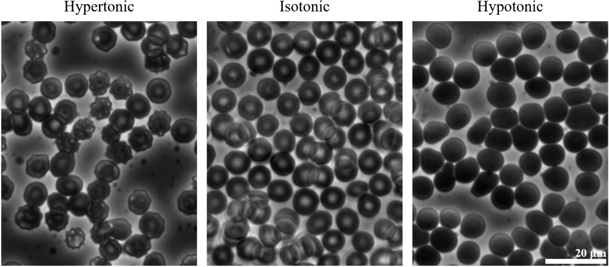
Fig. 5.5 Hypertonic solutions (high solute concentration, left) cause red blood cells to shrivel as water to leaves the cells, whereas hypotonic solutions (low solute concentration, right) cause water to enter the red blood cells so that the cells swell. An isotonic solution neither shrivels nor swells the cells and they retain their characteristic discoid appearance. (Image by Zephyris - Own work, CC BY-SA 3.0, [25].)
Fig. 5.6 illustrates the concept of osmotic pressure with an imaginary experiment in which a solution of liquid is surrounded by a semipermeable membrane and then submerged in pure solvent. The osmotic pressure \(\Pi\) is the pressure above ambient pressure that is just sufficient to stop the net influx of solvent from the surroundings into the solution.
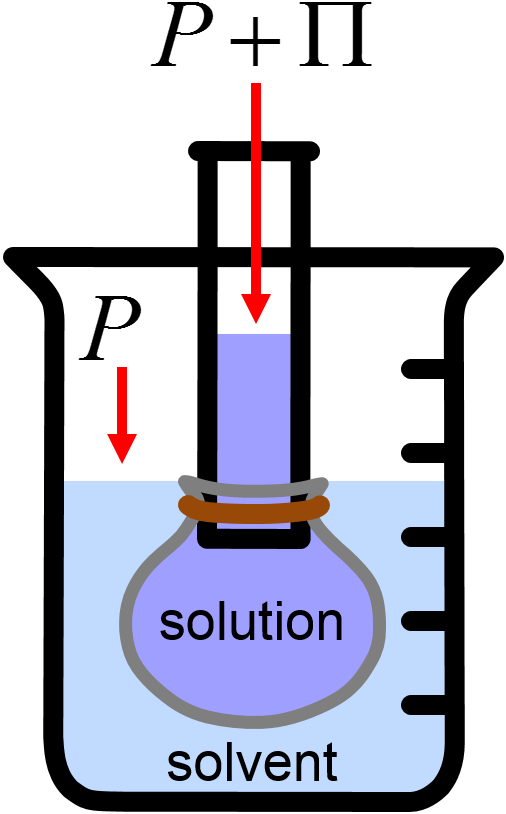
Fig. 5.6 Illustration of osmotic pressure with a semipermeable membrane that is permeable to solvent but not solute. Osmotic pressure is the minimum applied pressure \(\Pi\) that will stop the net flow of solvent from the surroundings (blue) to the solution (purple).
Under applied pressure \(\Pi\), the chemical potential of the solvent in the surroundings at ambient pressure \(P\) equals the chemical potential of the solvent in the solution at pressure \(P+\Pi\). We will refer to the solvent as A and the solute as B, and thermodynamic quantities that use the pure liquid or solid will linclude the symbol * for completeness.
For the right hand side of the above equation, we will use the ideal solution equation (Eq. (5.5)) to relate the solution chemical potential at pressure \(P+\Pi\) and temperature \(T\) to the solvent chemical potential at the same pressure and temperature.
Next, we can use our understanding of how Gibbs free energy changes with pressure to calculate the change in chemical potential for changing the pressure of the solvent. We found previously (Eq. (4.6)) that
and for a process at constant pressure we can thererfore relate chemical potenial to \(dG/n\) according to
This equation can be integrated to find the change in chemical potential when going from \(P\) to \(P+\Pi\)
where the approximation, above, is for the relatively good assumption that the volume of the pure liquid changes negligibly upon an increase in pressure. Using Eq. (5.10), we can relate this change in chemical potential for the pure solvent to \(RT\ln x_\textrm{A}\) according to
As for our freezing point depression derivation, above, we will assume a dilute solution consisting of mostly solvent A, where \(x_\textrm{A}\) is near 1
so that
Noting that \(n_\textrm{A}x_\textrm{B} = n_\textrm{B}\) we can rewrite the above equation in a form that looks almost identical to the ideal gas equation
or in terms of concentration of solute B, \(C_\textrm{B}\) as
It says that osmotic pressure is higher for higer concentrations and also for higher temperatures. The osmotic pressure relationship is simple and elegant. Let’s take a look at an example calculation.
Example 4: Calculate the osmotic pressure of Coca Cola at 298 K. Assume 110 g fructose (342.3 g/mol) per L of solution, with no other solutes, and \(T=298 \textrm{K}\).
Note that concentration, above, was converted to units of \(\textrm{mol/m}^3\) to be consistent with SI units. Now, I don’t know about you, but the first time I learned of the magnitudes of osmotic pressures for some common solutions, I found the values to be quite high. For reference, the ~8 atm is greater than the pressure of \(\ce{CO2}\) in a champagne bottle and approximately equal to the hydrostatic pressure at a depth of ~200 ft under water.
5.5.3. Colligative Properties and van’t Hoff Factor
In the above derivations and examples for colligative properties, the solutes were all considered not to dissociate so the number of moles of solute in solution is the same as the number of moles of solute that was added. But what if the solute dissociates? van’t Hoff realized that there would be a discrepancy in osmotic pressure for dissociating species, and that this also turns out to apply to freezing point depression and boiling point elevation. We can define the van’t Hoff factor, \(i\), as the ratio of number of moles of independent solute molecules in solution per mole of solute molecules added. For a salt like \(\ce{NaCl}\), which in water forms mostly dissociated \(\ce{Na+}\) and \(\ce{Cl-}\) ions the number of moles of solute in solution is about twice the number of moles of \(\ce{NaCl}\). For a salt like \(\ce{MgCl2}\), one would expect a three-fold increase. Species which don’t fully dissociate or which dimerize in solution could have a fractional value of \(i\).
We can revise our colligative properties equations by multiplying solute concentrations. These are presented in the next section together with an overall summary of equations from this chapter.
5.6. Summary of Key Equations
Here is a summary of key equations from this chapter for reference.
Equation |
Notes |
|---|---|
\(P_i=x_iP_i^*\) |
Raoult’s law |
\(\mu_i = \overline{G}_i = \dfrac{G}{n_i} = \left( \dfrac{\partial G}{\partial n_i} \right)_{P,T,n_{j\ne i}}dn_i\) |
chemical potential |
\(\mu_i(\textrm{solution}) = \mu_i^*(\textrm{liquid}) + RT\ln x_i\) |
ideal solution equation |
\(P_i = k_i x_i\) |
Henry’s law |
\(C_i = x_i\dfrac{n_\textrm{solvent}}{V_\textrm{solvent}}\) |
convert concentration to mole fraction for dilute solution |
\(C_\textrm{solute} = b_\textrm{solute} \rho_\textrm{solvent}\) |
relationship between concentration (mol/L) and molality (mol/kg) and solvent density for dilute solutions |
\(\Delta T = -iK_\textrm{F}b_\textrm{solute}\) |
freezing point depression |
\(K_\textrm{F} = \left| \dfrac{RT_\textrm{fus,A}^2 M_\textrm{A}}{\Delta H_\textrm{fus,A}^*/n_\textrm{A}} \right|\) |
freezing point depression constant |
\(\Delta T = iK_\textrm{B}b_\textrm{solute}\) |
boiling point elevation |
\(K_\textrm{B} = \left| \dfrac{RT_\textrm{vap,A}^2 M_\textrm{A}}{\Delta H_\textrm{vap,A}^*/n_\textrm{A}} \right|\) |
boiling point elevation constant |
\(\Pi = i\dfrac{n_\textrm{B}}{V}RT = iC_\textrm{B}RT\) |
osmotic pressure |
5.7. Additional Problems
5.7.1. Osmotic Pressure Practice
Assuming ideal behavior, calculate the following for a temperature of 298 K. A) The osmotic pressure of an aqueous saturated solution of \(\ce{NaCl}\) (6 M). B) How tall of a column of water would produce the osmotic pressure in part A)? (Reminder, \(P=\rho hg\).) C) What would the osmotic pressure be for a 6 M solution of \(\ce{MgCl2}\) assuming full dissociation (and sufficient solubility)?
Osmotic Pressure Practice, SOLUTIONS
Answers:
A) For this problem, be sure to be careful when handling the units carefully between \(R\) and \(n/V\). Here, I made sure to use consistent (SI) units, but just be careful whatever you decide to do here.
B) The height is surprisingly large. Again, I was careful to use SI units here to avoid getting into trouble.
so that
C) What is the van’t Hoff factor for \(\ce{MgCl2}\)? Expect full dissociation to 3 ions, so use \(i=3\). Since we already calculated osmotic pressure for sodium chloride at the same concentration in part A), let’s be lazy and just multiply the osmotic pressure for 6 M sodium chloride by the ratio of the van’t Hoff factors.