All these figures are based on OLR pentad and ECMWF 12-hour analyses during the period 1985-1997.
A few observations re MJOs and windspeed
- SOI and OLR intraseasonal RMS
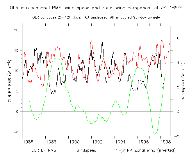
- OLR BP RMS and TAO windspeed and 1-yr RM zonal wind at 165°E
- OLR BP RMS and TAO modified windspeed 165°E
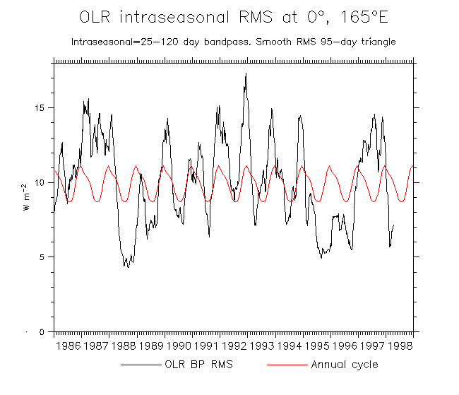
- OLR BP RMS with overlaid annual cycle at 165°E
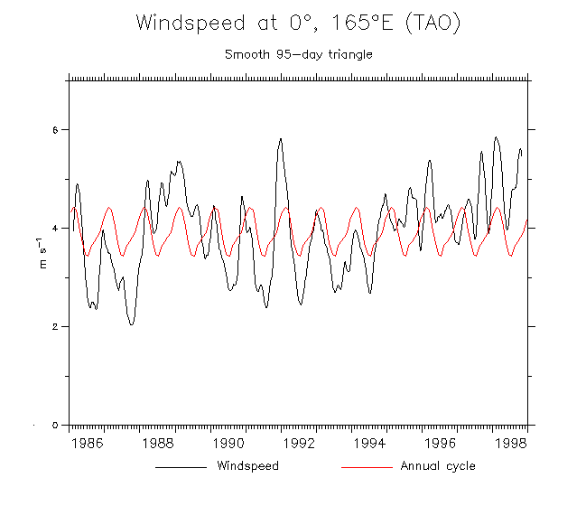
- TAO windspeed with overlaid annual cycle at 165°E
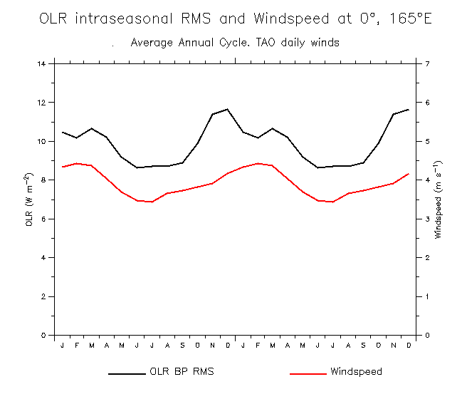
- OLR BP and TAO windspeed annual cycles compared at 165°E
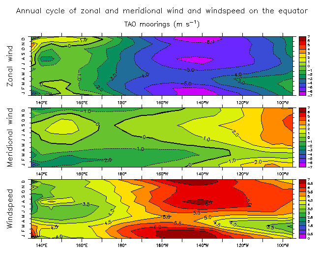
- TAO zonal/meridional wind and windspeed annual cycles on the equator
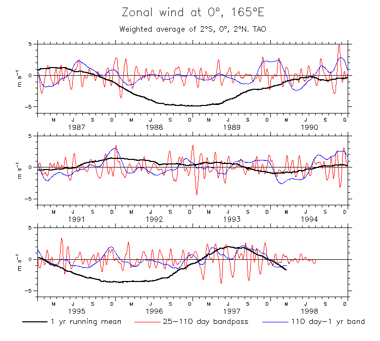
- TAO zonal wind at 0°, 165°E by frequency bands
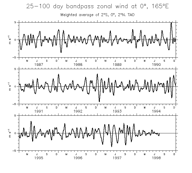
- TAO zonal wind at 0°, 165°E (25-110 day bandpass)
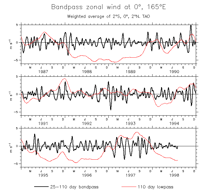
- TAO zonal wind at 0°, 165°E (25-110 day bandpass plus rest of low frequency)
- TAO zonal wind stress at 0°, 165°E (25-110 day bandpass plus rest of low frequency)
- Map of OLR bandpass intraseasonal RMS
Some varieties of the MJO experience
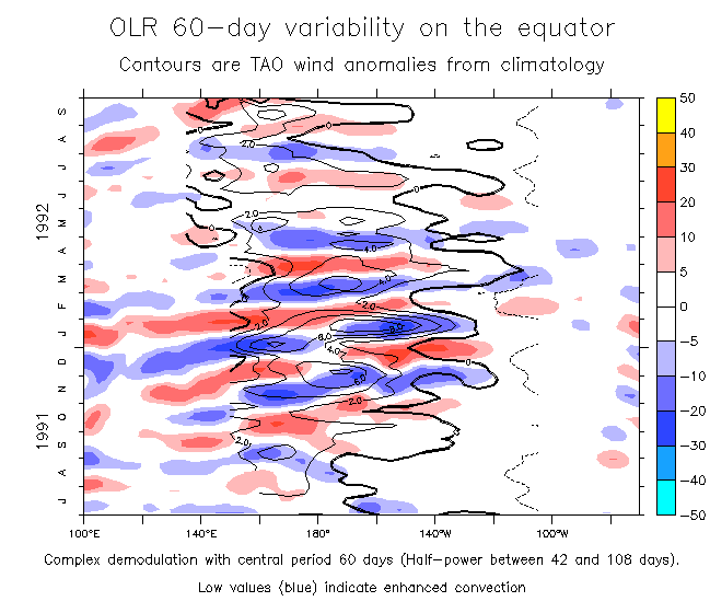
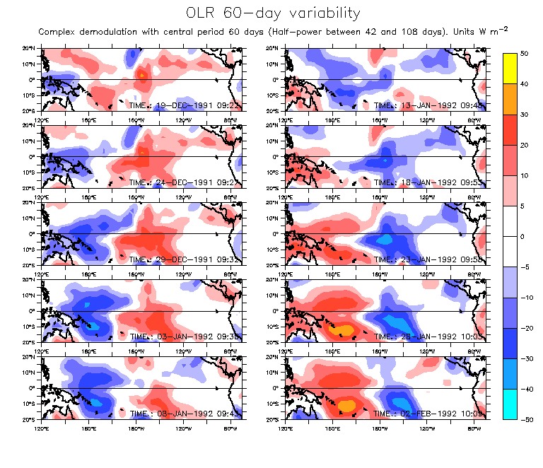
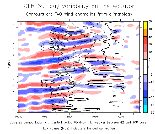
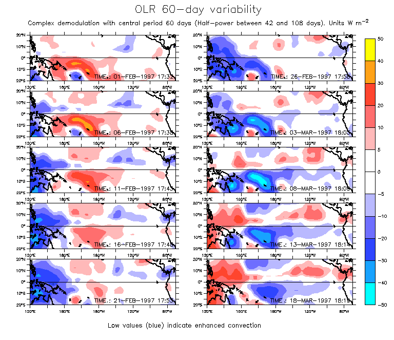
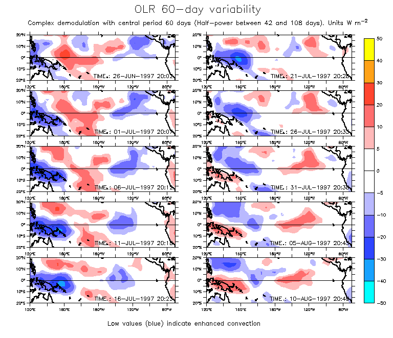
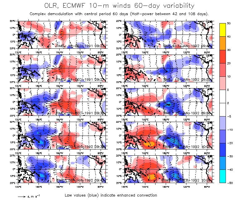
Examples of OLR variability at 60 day periods. This signal is extracted by complex demodulation on the OLR pentad time series. Half power of the filter is within 42-107 day periods. Low values (blue colors on the plots) indicates enhanced convection.
- Time series on the equator during 1991-92
- Example of evolution during November-December 1991
- Example of evolution during December 1991-January 1992
- Time series on the equator during 1997
- Example of evolution during February-March 1997
- Example of evolution during June-July 1997
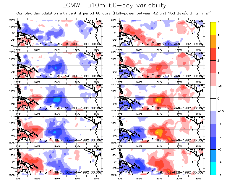
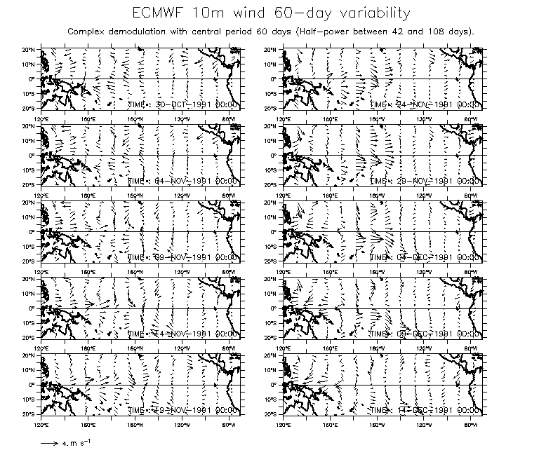
Some more examples from the ECMWF winds:
- Example of ECMWF zonal 10m wind evolution during November-December 1991
- Example of ECMWF zonal 10m wind evolution during December 1991-January 1992
- Example of ECMWF vector 10m wind evolution during November-December 1991
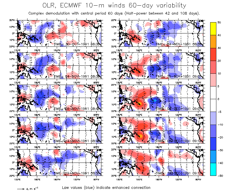
The same examples showing OLR and ECMWF wind vectors (a little hard to see but worth squinting at):
- Example of OLR and overlaid ECMWF vector 10m wind evolution during November-December 1991
- Example of OLR and overlaid ECMWF vector 10m wind evolution during December 1991-January 1992
Other useful things:
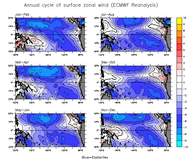
- The annual cycle of ECMWF (RA) zonal winds)
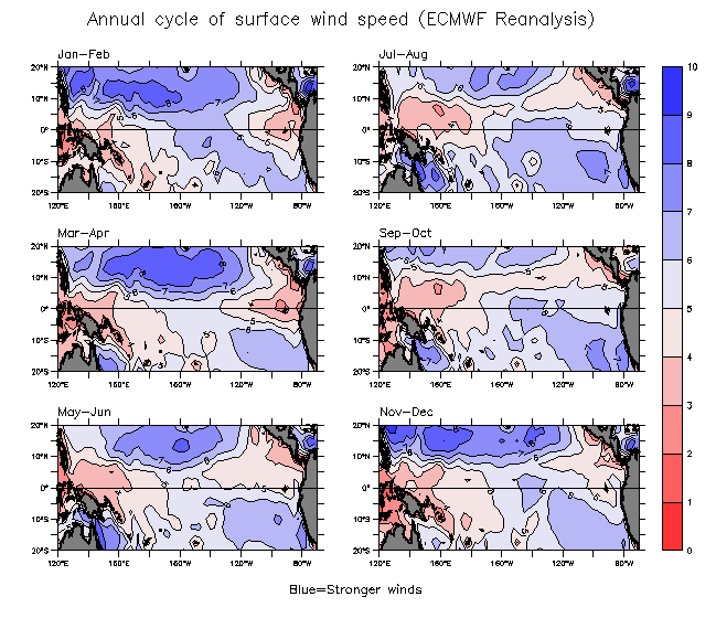
- The annual cycle of ECMWF (RA) windspeed)
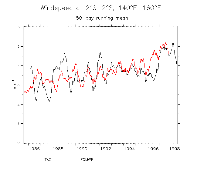
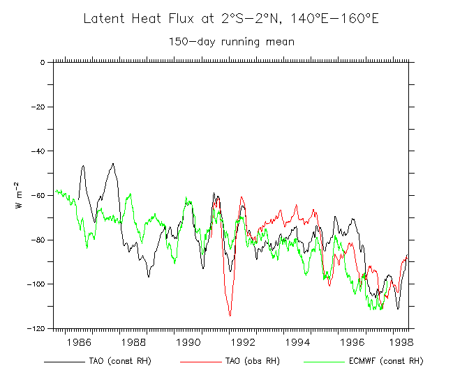
- The low-frequency trend in windspeed in the western equatorial Pacific (TAO and ECMWF)
- The low-frequency trend in latent heat flux in the western equatorial Pacific
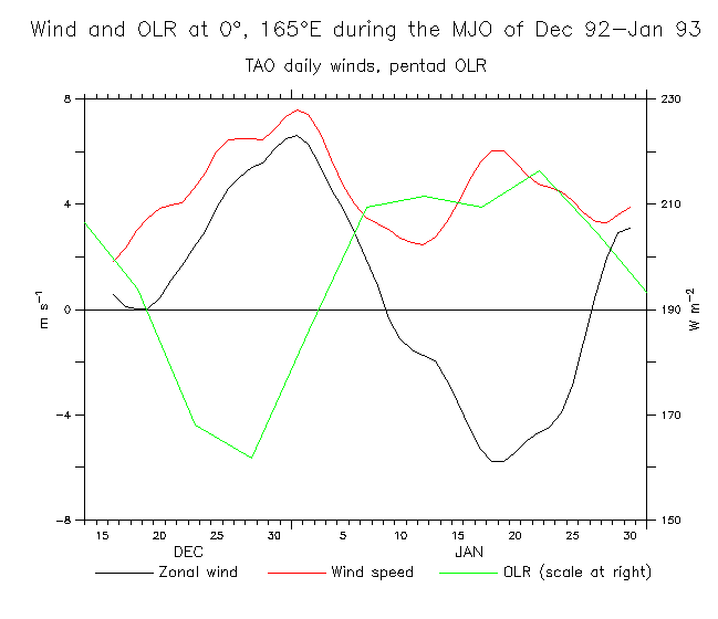
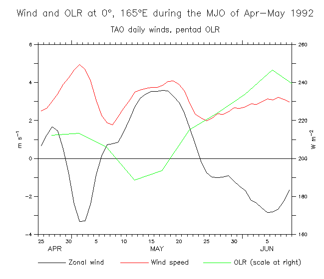
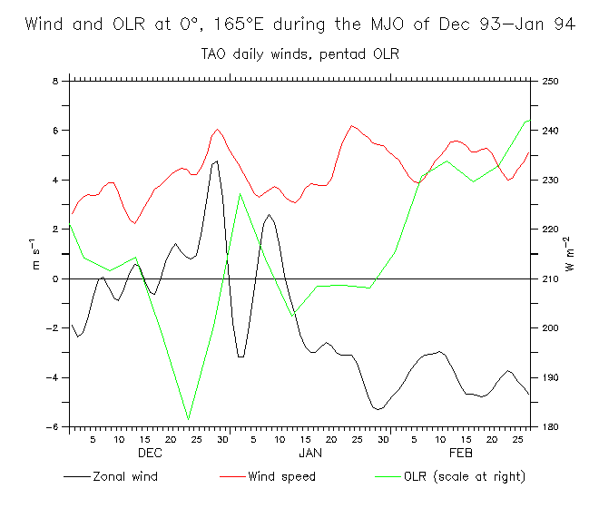
Some examples of OLR, zonal winds and windspeed during MJOs:
- Dec 92-Jan 93
- April-May 1992
- Dec 93-Jan 94
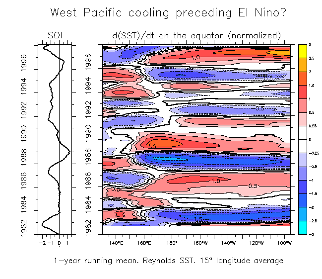
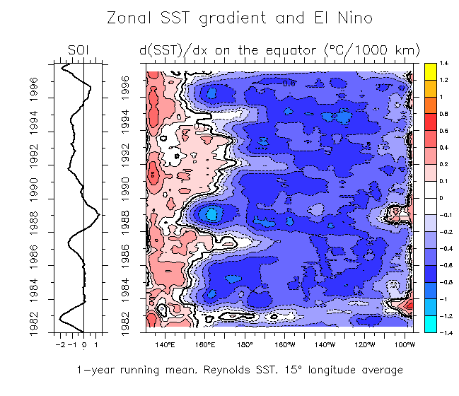
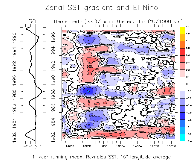
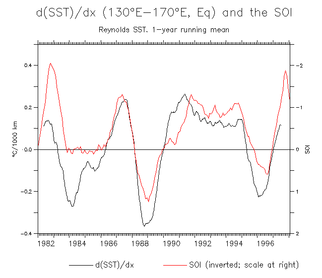
Cooling in the western Pacific preceding El Niño (and some other times, too):
- d(SST)/dt (Reynolds) and the SOI
- d(SST)/dx (Reynolds) and the SOI
- d(SST)/dx (demeaned) (Reynolds) and the SOI
- d(SST)/dx (130°E-170°E) (Reynolds) and the SOI
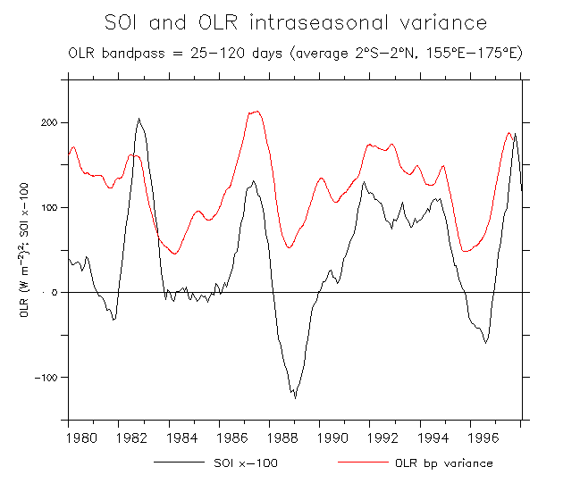
- SOI and OLR intraseasonal variance (Eq, WP)
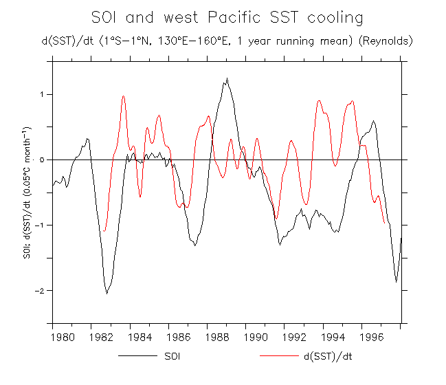
- SOI and west Pacific d(SST)/dt (Eq, WP)
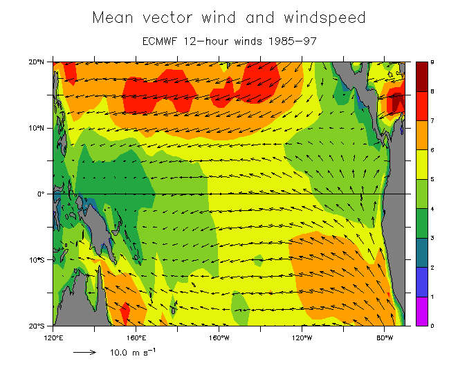
- ECMWF mean winds and windspeed
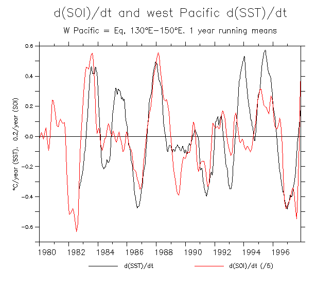
- WP d(SST/dt and d(SOI)/dt
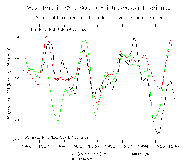
- WP SST, SOI and OLR BP RMS
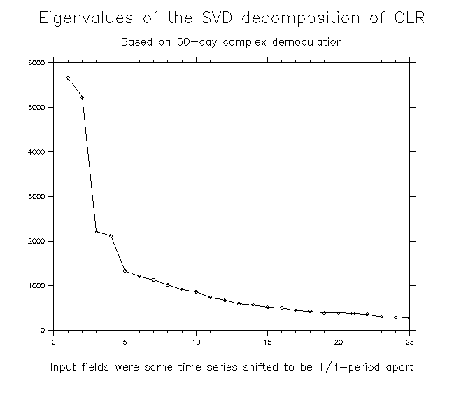
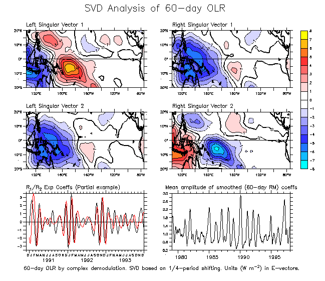
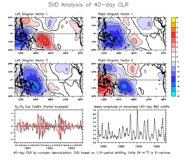
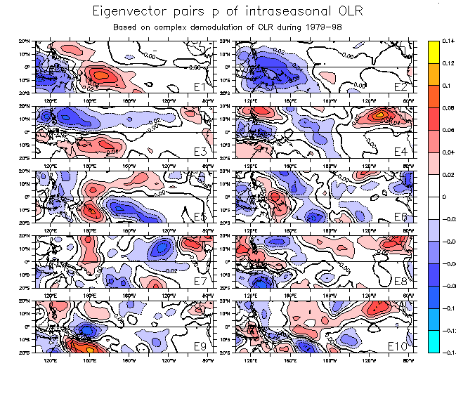
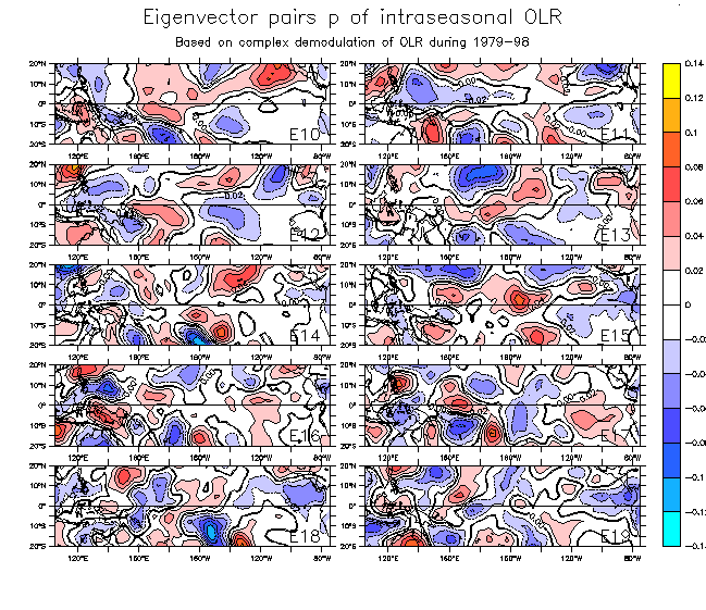
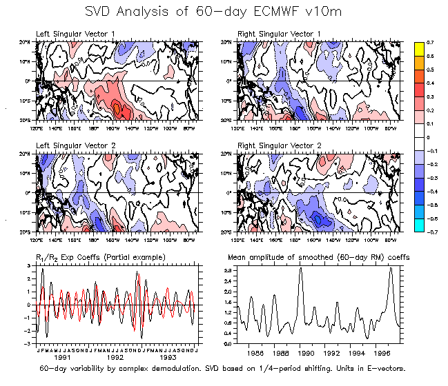
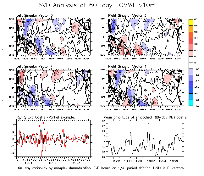
SVD analysis (Bretherton et al 1992) was used to decompose 60-day OLR reconstructed from complex demodulation (see first set of plots). Using an idea of Mike Wallace's, a second time series was formed by shifting the dates of the original by 15 days (1/4 period). The original and shifted time series were decomposed by SVD. The results give eigenvectors in quadrature pairs that represent propagating variability.
-
The SVD spatial patterns of 60-day OLR variability:
- First 25 eigenvalues of SVD modes of 60-day OLR
- SVD modes 1 and 2 of 60-day OLR
- SVD modes 3 and 4 of 60-day OLR
- SVD modes 1 and 2 of 40-day OLR
- SVD E-vectors 1-10 of 60-day OLR E-vectors 10-19
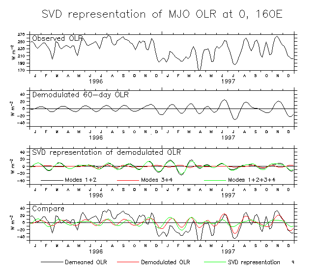
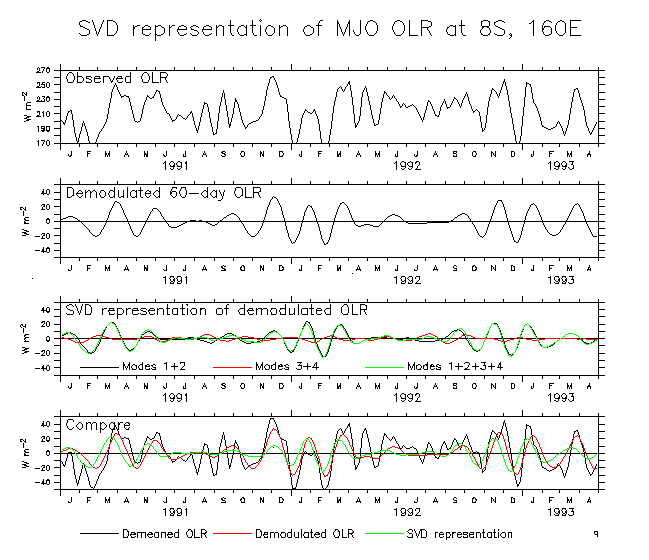
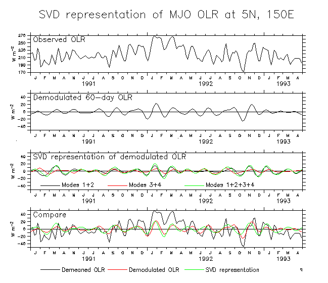
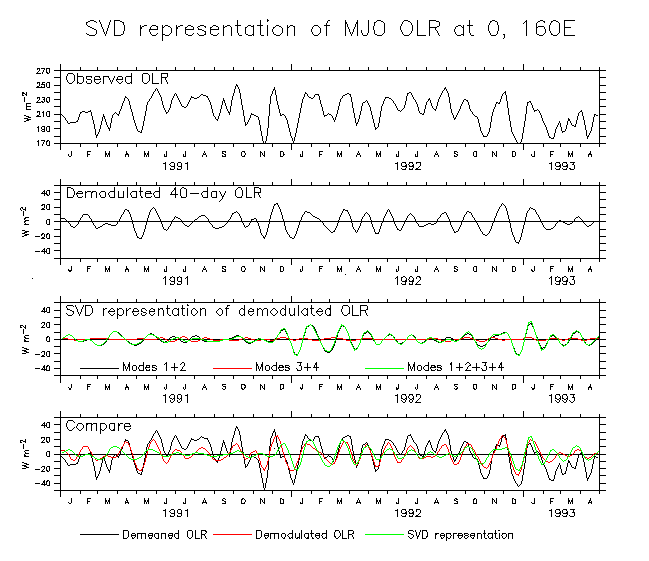
How well do complex demodulation and subsequent SVD represent MJO OLR?
- OLR 60-day variability at 0°, 160°E: SVD modes 1-4 (1991-93)
- OLR 60-day variability at 0°, 160°E: SVD modes 1-4 (1996-97)
- OLR 60-day variability at 8°S, 160°E: SVD modes 1-4 (1991-93)
- OLR 60-day variability at 5°N, 150°E: SVD modes 1-4 (1991-93)
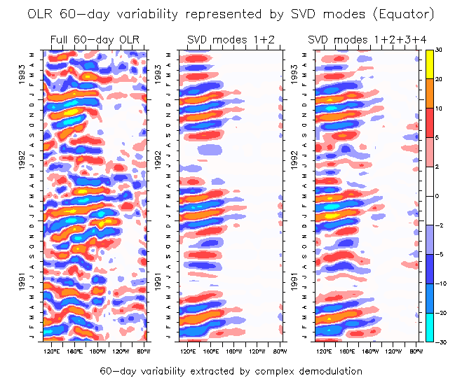
- OLR 60-day variability on the equator: SVD modes 1-4 (1991-93)
- OLR 60-day variability on the equator: SVD modes 1-4 (1996-97)
- OLR 40-day variability at 0°, 160°E: SVD modes 1-4 (1991-93)
What does an idealized (canonical?) MJO look like in OLR?
Represent this by SVD spatial patterns, assuming a purely sinusoidal time series. - Idealized OLR 60-day evolution: SVD modes 1+2
- Idealized OLR 60-day evolution: SVD modes 3+4
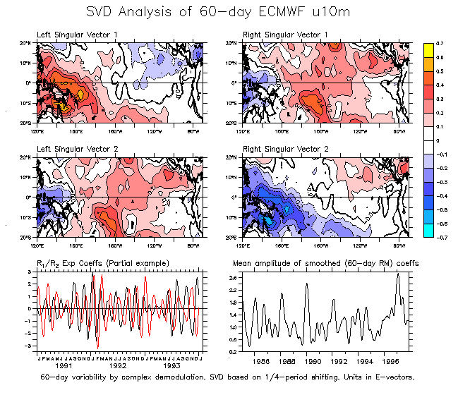
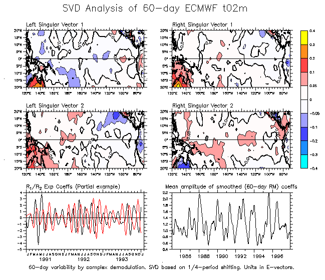
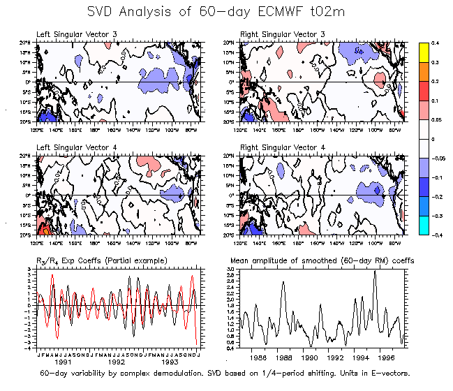
A similar complex demodulation-SVD technique was used to describe relevant terms from the ECMWF analysis. Zonal and meridional 10-meter wind components (labeled u10m and v10m) and 2-meter air temperature (t02m) were decomposed.
-
The SVD spatial patterns of 60-day OLR variability:
- U10m
- V10m
- T02m
SVD mode spatial patterns:
- Modes 1 and 2 of 60-day U10m
- Modes 3 and 4 of 60-day U10m
- Modes 1 and 2 of 60-day V10m
- Modes 3 and 4 of 60-day V10m
- Modes 1 and 2 of 60-day T02m
- Modes 3 and 4 of 60-day T02m
How well do complex demodulation and subsequent SVD represent ECMWF quantities?
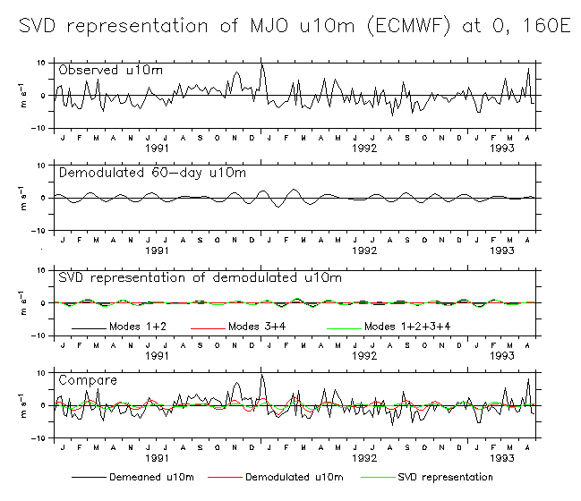
- U10m 60-day variability at 0°, 160°E: SVD modes 1-4(1991-93)
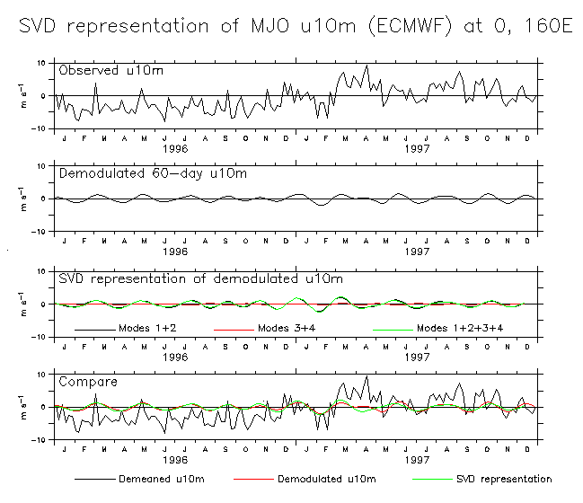
- U10m 60-day variability at 0°, 160°E: SVD modes 1-4 (1996-97)
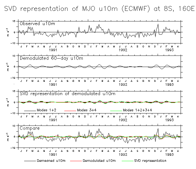
- U10m 60-day variability at 8°S, 160°E: SVD modes 1-4 (1991-93)
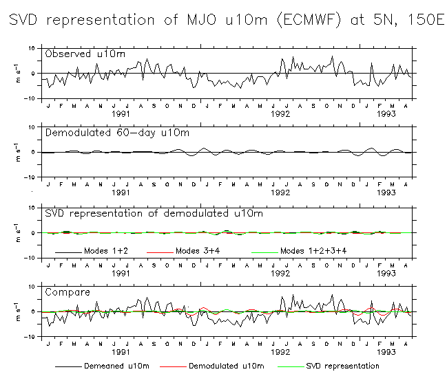
- U10m 60-day variability at 5°N, 150°E: SVD modes 1-4 (1991-93)
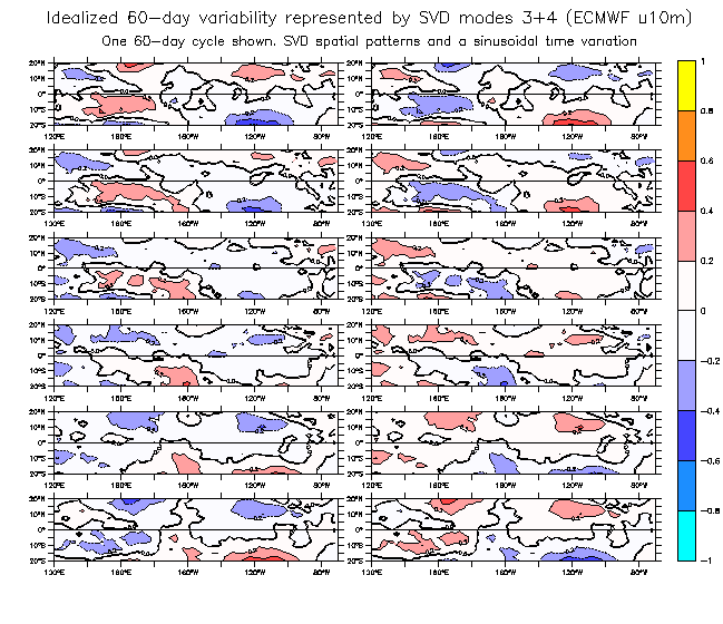
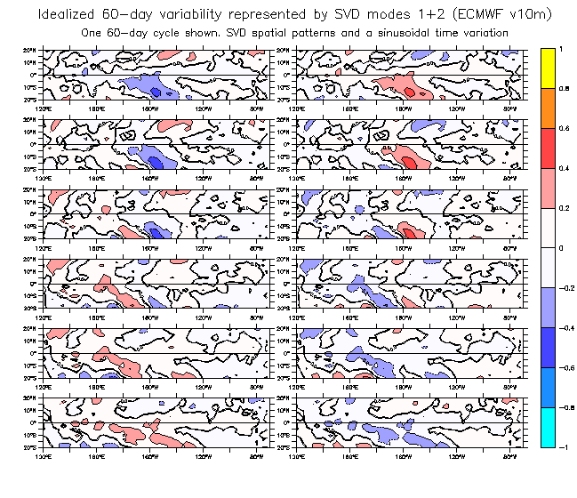
What does an idealized (canonical?) MJO look like in 10-meter winds?
Represent this by SVD spatial patterns, assuming a purely sinusoidal time series. - Idealized U10m 60-day evolution: SVD modes 1+2
- Idealized U10m 60-day evolution: SVD modes 3+4
- Idealized V10m 60-day evolution:y SVD modes 1+2
The 2-meter temperature decomposition was not satisfactory for this purpose since it is dominated by changes over land (Australia). See figs 8-9.
The other problem with this method is that there is no way to establish the phase relation between OLR and the wind fields (or for that matter between the zonal and meridional components of the winds themselves. Therefore this will be of limited usefulness in developing a picture of the total MJO.
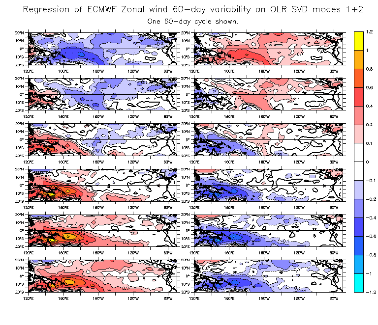
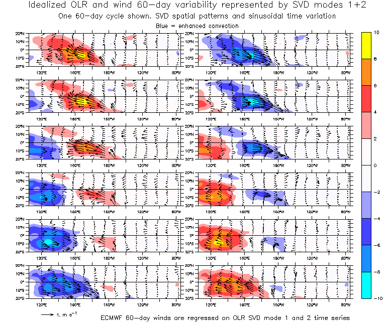
Try another method. Regress the ECMWF 60-day winds on the OLR SVD mode time series. Do the regression as a function of lag (since both time series are band-passed to 60-day periods). That produces an average 60-day cycle of winds that is fixed to the OLR phase.
- ECMWF U10m 60-day variability regressed on OLR SVD modes 1+2
- ECMWF vector wind 60-day variability regressed on OLR SVD modes 1+2
- OLR and ECMWF vector wind 60-day variability. Wind regressed on OLR SVD modes 1+2
- OLR and ECMWF vector wind 40-day variability. Wind regressed on OLR SVD modes 1+2
First 25 SVD eigenvalues of ECMWF 60-day quantities:
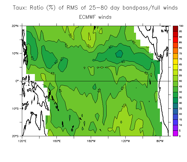
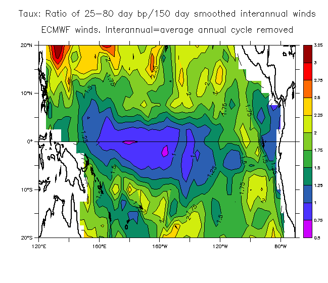
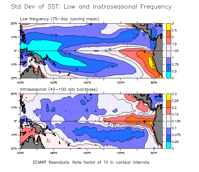
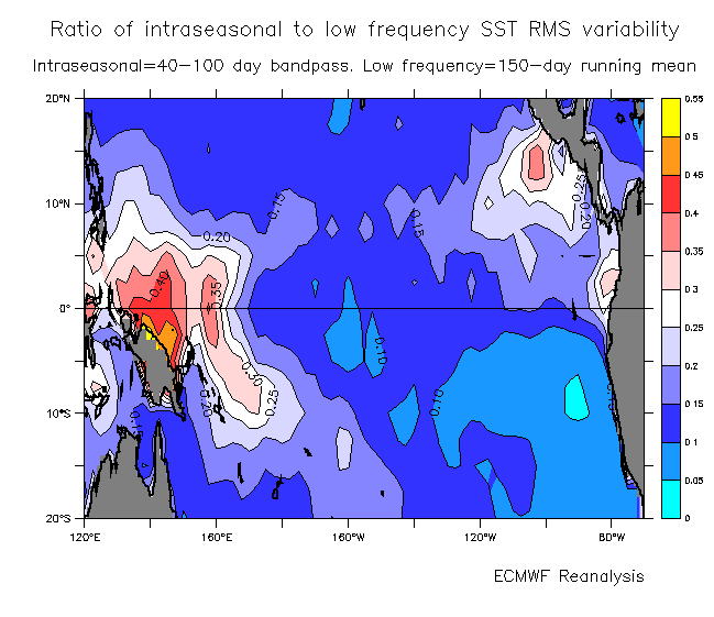
ECMWF heat/momentum flux terms.
The terms are made from the ECMWF 12-hour analysis. The terms are found from bulk formula based on ECMWF winds, SST, and air temperature (not the ECMWF fluxes themselves). Clouds are estimated by a regression from OLR (that means that only convective clouds are represented). Constant humidity of 75% is assumed. Therefore these calculations are very crude!
Various ways of looking at these are displayed. Ratios of the RMS amplitude of zonal wind stress in different frequency bands.
- 25-80-day bandpass/full winds
- 25-80-day bandpass/full winds smoothed with a 150-day running mean
- 25-80-day bandpass/interannual winds winds
- 25-80-day bandpass/interannual winds smoothed with a 150-day running mean
- Standard deviation of SST for low and intraseasonal frequencies
- Ratio of SST RMS variability for low and intraseasonal frequencies
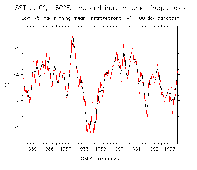
- Example of SST (0,160°E) in low and intraseasonal bands
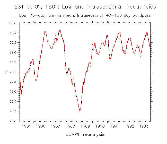
- Example of SST (0,180°) in low and intraseasonal bands
- Short wave radiation
- Long wave radiation
- Latent Heat Flux
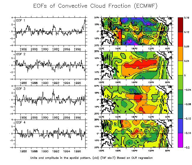
- Cloud fraction (convective clouds only)
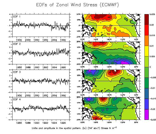
- Zonal wind stress
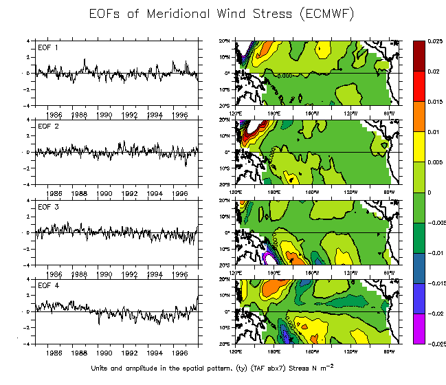
- Meridional wind stress
A page of TAO statistics for latent heat flux observables
A page for comparing clouds and OLR
Return to the main figures page
 |
Dr. William S. Kessler
NOAA / PMEL / OCRD 7600 Sand Point Way NE Seattle WA 98115 USA |
Tel: 206-526-6221
Fax: 206-526-6744 E-mail: william.s.kessler@noaa.gov |
| See also: | Kessler home page Kessler publications PMEL home page | |