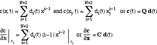
Orthogonal Collocation Method

The method of orthogonal collocation expands the solution in orthogonal polynomials in x, in the same way that was done for boundary value problems. Now the coefficients depend on time.

It is possible to derive the same spatial derivatives evaluated at the collocation points.

Now both c and ðc/ðx are functions of time, but the matrix A is constant in time. For the time derivatives we have

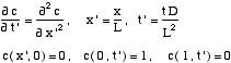
Consider the following diffusion problem.

Make it nondimensional since the orthogonal polynomials are defined on x = (0,1),

The orthgonoal collocation formulation is

This problem can be integrated using the standard methods for ordinary differential equations as initial value problems. One problem, though, is that one has N ordinary differential equations which depend upon N+2 variables. Two of the variables are determined by the boundary conditions. When solving the problem with Matlab, it is necessary to solve for the N derivatives, given the N variables. The other two variables must be known or determined.

Here the boundary conditions are

Thus, in the function defining the right-hand side of the equation, it is a simple matter to provide values for c₁ and c_N+2, which come from the boundary conditions. The algorithm, though, looks like this:

Given y(1),...,y(N)
Put c(i+1) = y(i), i = 1,...,N (Now we have the points c₂ through c_N+1 ,)
Assign c(1) = c₁, and c(N+2) = c_N+2,
Compute the right-hand sides for dc_j/dt, j=2,...,N+1.
Put the values in dy(j)/dt = dc_j+1/dt, j=1,...,N.
Return dy(j)/dt to the program

The method is illustrated using the following code (which relies on the code planar.m to generate the orthogonal collocation matrices). The solution using 7 collocation points is shown in Figure 1. The solution is just plotted with straight lines between the solution at collocation points, and it is clear ragged. This is typical when trying so solve a transient problem, close to a discontinuity (i.e. close to t = 0). The plot using a spline interpolation of the collocation solution is in Figure 2. This shows that there are even negative values in the interpolated values. While the collocation solution is fine for times greater than t = 0.1, it is clearly irregular and unsatisfactory for times t = 0.01 and below. In those cases, it is necessary to either use a method with piecewise approximation (finite difference; orthogonal collocation on finite elements; or finite element method); or provide an added function encorporating the small-time solution, as was done in the Method of Weighted Residuals.

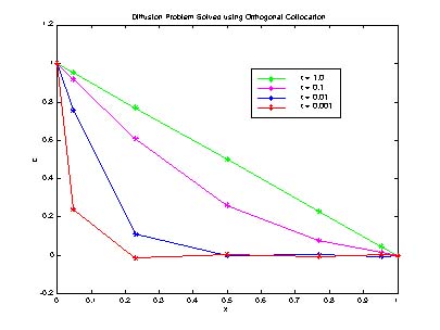
Figure 2. Orthogonal Collocation Solution, N = 7

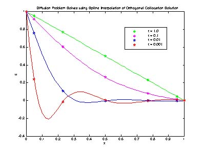
Figure 3. Orthogonal Collocation Solution, N = 7, Spline Interplation

If one of the boundary conditions is changed to

what do we do? In that case we can either solve for the N+2-th variable inside the algorithm

or we can solve for it and substitute it into the differential equations. In that case we get

Either method makes it easy to use the standard integrators in numerical packages.

Next consider the case when the diffusivity depends upon concentration, D(c). There are two ways to approach this problem. The first one is to differentiate the equation

and then apply orthogonal collocation.

The second one is to apply orthogonal collocation for first derivatives twice.

This equation can be written in the form

Separation of Variables
Combination of Variables
Numerical Methods - Overview
Finite Difference Methods in MATLAB
Orthogonal Collocation on Finite Elements
Finite Element Method
Method of Weighted Residuals
Spectral Methods
Errors
Stability
Comparison of Methods