Method of Weighted Residuals
The method of weighted residuals can solve partial differential equations. The method is a slight extension of that used for boundary value problems. We apply it in five steps:
1. Expand the unknown solution in a set of basis functions, with unknown coefficients or parameters; this is called the trial solution.
2. Make the trial solution satisfy the boundary conditions (usually) and initial conditions (perhaps in a MWR sense).
3. Define the residual.
4. Set the weighted residual to zero and solve the equations.
5. Examine the error by constructing successive approximations, and show convergence as the number of basis functions increases.
We apply the method to a simple diffusion problem.
![]()
The solution is expanded in the series (step 1)
![]()
We choose c0(x) to satisfy the nonhomogeneous boundary conditions.
![]()
The simplest form is
![]()
Next we choose the ci(x) to satisfy the homogeneous boundary conditions.
![]()
Possible choices are
Now the trial solution satisfies the boundary conditions (part of step 2). Consider the first choice and postpone the satisfaction of the initial conditions. The residual is defined (step 3)
![]()
The weighted residual is set to zero (step 4); here we use the Galerkin criterion and make the residual orthogonal to each member of the basis set, sin jx.
![]()
This gives
![]()
This is zero if
![]()
i.e. if
![]()
The combined solution is then
![]()
The constants Ai(0) are obtained by applying the Galerkin method to the initial residual c(x,0) = 0.
![]()
This gives (link)
![]()
Thus, we get the same solution as derived by separation of variables. Thus, the Galerkin method applied to linear problems gives the first N terms of the exact solution found by separation of variables when the expansion functions are the exact eigenfunctions.
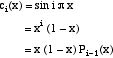
Next, we make the choice (part of step 2)
![]()
Then the derivatives of ci(x) are
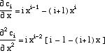
and the residual is (step 3)
![]()
We make the residual orthogonal to each member of the basis set, xj( 1 x ) (step 4, using the Galerkin method).
![]()
These equations can be written in the format
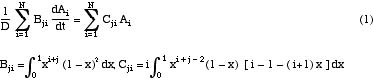
which can be solved with matrix methods or numerically. We note that the only difference between this solution and the previous one is the choice of trial function - sine functions versus polynomials - making the matrices different. Because the sine functions are the exact eigenfunctions, the equations for Ai(t) simplify to a series of single equations easily solved (this is a property of the exact eigenfunctions). With the polynomial functions, the polynomial basis functions are not orthogonal to each other, and all the equations are coupled together.
We know that the solution obtained by separation of variables requires lots of terms for small times, and we expect the same to be true for the MWR solution derived in the way given above. For longer times, however, the separation of variables solution requires only a few terms, maybe only one, and this is true of the MWR solution, too. Thus, the accuracy depends upon the number of terms kept in the series as well as the time interval over which you are interested in the solution.
For a single term, with MWR we have
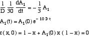
Applying the Galerkin method to the initial condition gives A1(0) = 2.5. The complete solution is
![]()
We expect this solution to be valid only for long time.
If we want to solve the problem for small time, increasing to larger time, then we can combine MWR with the solution by combination of variables (link). We know for small time the solution is
![]()
This solution applies for an infinite domain, and it is valid provided the concentration at the far boundary does not depart too much from zero (say 10-6). We employ MWR by writing the solution as the sum of this function plus another function to be determined (step 1).
![]()
The function u(x,t) must satisfy
We use polynomials for the function u(x,t) and must satisfy the boundary conditions (step 2)
![]()
A quadratic function which does that is
![]()
The initial condition is satisfied if we take A(0) = 0 (the rest of step 2). The residual is (step 3)
![]()
where
![]()
The Galerkin weighted residual (step 4) is
![]()
The function A(t) is the solution to
![]()
The complete solution is shown in the figure and is a good approximation for all times. The exact and approximate solutions are indistinguishable on the graph.
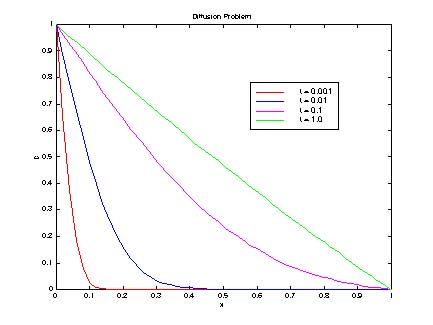
Solution to Diffusion Problem using MWR combined with the small time solution
The same ideas can be applied to nonlinear problems when no separation of variables solution
exists (Finlayson, 1980, p. 187). To solve nonlinear problems, and higher approximations, one would
use computer packages to solve sets of initial value problems. The packages would have to permit
the matrix on the left hand side of Eq. (1) above.
Separation of Variables
Combination of Variables
Numerical Methods - Overview
Finite Difference Methods in MATLAB
Orthogonal Collocation Methods
Orthogonal Collocation on Finite Elements
Finite Element Method
Spectral Methods
Errors
Stability
Comparison of Methods
Take Home Lesson: The Method of Weighted Residuals provides a simple method for deriving approximate solutions to partial differential equations. Higher order approximations would be derived numerically, and it is simpler then to use one of the other methods.