Finite Element Method

The finite element method is handled as an extension of two-point boundary value problems by letting the solution at the nodes depend on time. For the diffusion equation the finite element method gives

with the mass matrix defined by

The B matrix is derived elsewhere. This set of equations can be written in matrix form

Now the matrix CC is not diagonal, so that a set of equations must be solved each time step, even when the right-hand side is evaluated explicitly. This is not as time-consuming as it seems, however. Write the explicit scheme as

Compute the right-hand side vector in the usual way, calling it f_j, and then solve

Solve with an LU decomposition which retains the structure of the mass matrix CC. Thus

At each step then calculate

This is quick and easy to do since the inverse of L and U are simple. Furthermore, they do not change with time, and the LU decomposition need be done only once per problem. Thus the problem is reduced to solving one full matrix problem and then evaluating the solution for several right-hand sides.

An alternative is to use the packages which allow for the matrix on the left-hand side of the equation.

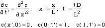
To illustrate the procedure, we take the problem

and apply the Galerkin finite element method using linear trial functions. The element diffusion matrix is then

and the element mass matrix is

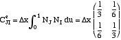
These matrices are combined element by element to form the global matrix. For four elements we get for the right-hand side

The first and last row are deleted since the first and last variables are determined by the boundary conditions. The mass matrix is

The first and last row and column are deleted since they are not used. We use the following algorithm inside the function defining the right-hand side.

Given y(1),...,y(NT­2)
Put c(i+1) = y(i), i = 1,...,NT­2 (Now we have the points c₂ through c_NT­1 ,)
Assign c(1) = c₁, and c(NT) = c_NT,
Compute the right-hand sides for f_j, j=1,...,NT­2 (for derivatives dc_j+1/dt, j=1,...,NT­2)
If using the LU decomposition, perform the fore and aft sweep of the LU decomposition
Or, if using a code allowing for CC, calculate CC, too.
Return dy(j)/dt to the program

Figure 1 shows the correspondence between the variables y(internal to the program) and the variables c.

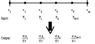
Figure 1. Nodal Numbering and Unknown Numbering

The code is available. Typical solutions are shown in Figure 2 (for four elements) and Figure 3 (for eight elements) and Figure 4 (for sixteen elements. The first nodal point shows a negative value at small time, but this becomes positive as the solution progresses. This effect is made smaller as x is decreased (compare Figures 2-4). Also, as x gets smaller, the problem becomes stiffer (link) and an explicit scheme is less effective. Switching to ode15s provided the solution much faster than ode45. This code used the LU decomposition for tridiagonal matrices, which is much faster than using a LU decomposition for dense matrices.

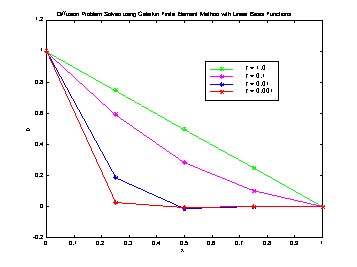
Figure 2. Diffusion Problem with 5 nodes, x = 0.25

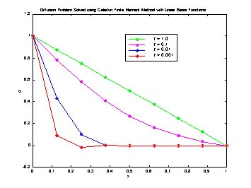
Figure 3. Diffusion Problem with 9 nodes, x = 0.125

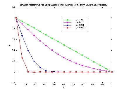
Figure 4. Diffusion Problem with 17 nodes, x = 0.0625

The Galerkin finite element method can be applied when the diffusivity depends upon the concentration. In that case, it is necessary to include the diffusivity in the matrix B. Typically, the integral is evaluated using Gaussian quadrature, which is very accurate when using only a few terms.
Separation of Variables
Combination of Variables
Numerical Methods - Overview
Finite Difference Methods in MATLAB
Orthogonal Collocation Methods
Orthogonal Collocation on Finite Elements
Method of Weighted Residuals
Spectral Methods
Errors
Stability
Comparison of Methods