Collocation and Orthogonal Collocation
The orthogonal collocation method has found widespread application in chemical engineering, particularly for chemical reaction engineering. We first discuss the collocation method [Finlayson, 1972, 1980], and then show the changes to make it the orthogonal collocation method. The dependent variable is expanded in a series.
![]() (1)
(1)
Suppose the differential equation is
![]()
Then the expansion is put into the differential equation to form the residual.
![]()
In the collocation method the residual is set to zero at a set of points, called collocation points.
![]()
This provides N equations; two more equations come from the boundary conditions, giving N+2 equations for N+2 unknowns. This procedure is especially useful when the expansion is in a series of orthogonal polynomials, and when the collocation points are the roots to an orthogonal polynomial, as first used by Lanczos [1938, 1956]. A major improvement was proposed by Villadsen and Stewart [1967], who proposed that the entire solution process be done in terms of the solution at the collocation points rather than the coefficients in the expansion. Thus we would evaluate Eq. (1) at the collocation points
![]()
and then solve for the coefficients in terms of the solution at the collocation points.
![]()
Furthermore if we differentiate Eq. (1) once, and evaluate it at all collocation points, we can write the first derivative in terms of the values at the collocation points.
![]()
This can be written as
![]()
or shortened to
![]()
Similar steps can be applied to the second derivative to get:
![]()
We next apply this method to the differential equation for reaction in a tubular reactor, after the equation has been made nondimensional so that the dimensionless length is 1.0.
![]() (2)
(2)
The differential equation at the collocation points is
![]() (3)
(3)
and the two boundary conditions are
![]() (4)
(4)
Note that 1 is the first collocation point (x=0) and N+2 is the last one (x=1). To apply the method it is neccessary to find the matrices Aij and Bij and then solve the set of algebraic equations, perhaps with the Newton-Raphson method. If orthogonal polynomials are used, and the collocation points are the roots to one of the orthogonal polynomials, then we get what is known as the orthogonal collocation method.
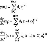
In the orthogonal collocation method we expand the solution in a series involving orthogonal polynomials, usually Legendre polynomials.
![]() (5)
(5)
which is also
![]()
The collocation points are shown in the figure. There are N interior points plus one at each end. and the domain is always transformed to lie on 0 to 1. To define the matrices Aij and Bij we evaluate this expression at the collocation points; we also differentiate it and evaluate the result at the collocation points.
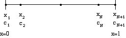
Figure: Orthogonal Collocation Points
Put these formulas in matrix notation, where Q, C, and D are N+2 by N+2 matrices.
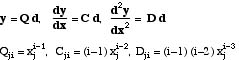
Solving the first equation for d we can rewrite the first and second derivatives as
![]() (6)
(6)
Thus the derivative at any collocation point can be determined in terms of the solution at the collocation points. The same property is enjoyed by the finite difference method and the finite element method (link), and this property accounts for some of the popularity of the orthogonal collocation method. To apply the method to Eq. (2) we get the same result, Eq. (3) and (4), with the matrices defined in Eq. (6). If we wish to find the solution at a point that is not a collocation point then we use Eq. (5); once we know the solution at all collocation points we can find d, and once we know d we can find the solution for any x.
To evaluate integrals accurately, we use the quadrature formula
![]()
To determine Wj we evaluate this equation for powers of x.
![]()
![]()
This is Gaussian quadrature.
To use the orthognal collocation method we need the matrices. They can be calculated as shown above for small N (N<8 or so) and using more rigorous techniques for higher N. It is useful, however, to have the matrices listed explicitly for N = 1 and 2, which are shown in Table I. An application to a nonlinear heat transfer problem is provided.
Orthogonal collocation can be applied to distillation problems. Stewart, et al. [1984] and [Stewart, et al., 1985] develop a method using Hahn polynomials which retains the discrete nature of a plate-to-plate distillation column. Other work treated problems with multiple liquid phases [Swartz and Stewart, 1987].