Spectral Methods

Spectral methods employ Chebyshev polynomials and the Fast Fourier Transform and are quite useful for hyperbolic or parabolic problems on rectangular domains[Gottlieb and Orszag, 1977]. The Chebyshev polynomial of degree n is defined by

The first few polynomials are

They satisfy the orthogonality condition

where the constants are given by

When solving a differential equation for f(x,t), for example, the function f is expanded in Chebyshev polynomials

Various derivatives are also expanded in Chebyshev polynomials. For differential operator L we write formally

For specific cases [Gottlieb and Orszag, p. 160, 1977] the relations between the coefficients of the function (a_n ) and the derivatives (b_n) are given by

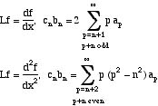
Derivatives can be evaluated even more efficiently using a recursion relation. When

we can use [Gottlieb and Orszag, p. 117, 1977]

This recurrence relation is assured by

In the Chebyshev collocation method we use the N+1 collocation points

As an example, consider the equation

We use an explicit method in time

and evaluate this at each collocation point

The trial function is taken as

(1)

We assume that we have values u_jⁿ at some time. Then we invert equation (1) using the fast Fourier transform to obtain {a_p} for p = 0, 1, ..., N. We then calculate S_p

and finally

Thus the first derivative is given by

This is evaluated at the set of collocation points by using the fast Fourier transform again. Once the function and the derivative is known at each collocation point the solution can be advanced forward to the n+1-st time level.

The advantage of the spectral method is that it is very fast and can be adapted quite well to parallel computers. It is, however, restricted in the geometries that can be handled.